CEI Comments on EPA Proposed Rule “Reconsideration of 2009 Endangerment Finding and Greenhouse Gas Vehicle Standards”

Dear Mr. Stout:

On behalf of the Competitive Enterprise Institute (CEI), we appreciate this opportunity to provide comments on the Environmental Protection Agency’s (EPA) proposed rule “Reconsideration of 2009 Endangerment Finding and Greenhouse Gas Vehicle Standards.” It required strong leadership and courage to reconsider the Endangerment Finding given the constant and vocal attacks on anyone that would even dream of challenging the finding. To the EPA’s credit, the agency is demonstrating this leadership and courage. For that we commend you.

Our comment starts with some general points including those connected to the proper interpretation of Section 202(a) of the Clean Air Act. The next section discusses why Section 202(a) does not authorize greenhouse gas vehicle standards. We then discuss some additional issues, including a section specifically applicable to the Biden EPA’s standards for Model Year (MY) 2027 and Later Light-Duty and Medium-Duty Vehicles. Finally, we close out our comment with an extensive discussion of climate science and its relationship to this rulemaking.

I. General Points

Proper interpretation of Section 202(a). It helps to start with laying out the relevant statutory language for determining whether greenhouse gas emission vehicle standards are authorized.

Section 202(a) of the Clean Air Act states:

• Authority of Administrator to prescribe by regulation Except as otherwise provided in subsection (b)—
  • The Administrator shall by regulation prescribe (and from time to time revise) in accordance with the provisions of this section, standards applicable to the emission of any air pollutant from any class or classes of new motor vehicles or new motor vehicle engines, which in his judgment cause, or contribute to, air pollution which may reasonably be anticipated to endanger public health or welfare. Such standards shall be applicable to such vehicles and engines for their useful life (as determined under subsection (d), relating to useful life of vehicles for purposes of certification), whether such vehicles and engines are designed as complete systems or incorporate devices to prevent or control such pollution.
  • Any regulation prescribed under paragraph (1) of this subsection (and any revision thereof) shall take effect after such period as the Administrator finds necessary to permit the development and application of the requisite technology, giving appropriate consideration to the cost of compliance within such period.

Language within 202(a), such as “new” or “class or classes,” may not simply be read out of the statute or be read in isolation as if it does not work together with the other language within the section. It requires the agency, to among other things, prescribe standards for emissions of an air pollutant from any class or classes of new motor vehicles or new motor vehicle engines. Ignoring any of these terms is ignoring the clear requirements of the statute.

As explained in the Proposed Rule, the Endangerment Finding severed “the question whether GHG emissions from new motor vehicle engines contribute to GHG concentrations in the atmosphere from the question whether GHG concentrations in the atmosphere endanger public health and welfare.” The reading of the statute in such a manner may have helped the EPA get an outcome it desired, but it is in direct conflict with the plain language of the statute. The analysis regarding the contribution of emissions is connected to the effect those emissions have on the air pollution and specifically the alleged harm caused by that air pollution.

The language in Section 202(a) also requires that the agency when deciding whether emissions “cause or contribute” to air pollution that may reasonably be anticipated to endanger public health or welfare look at emissions from new motor vehicles or new motor vehicle engines, not emissions from existing vehicles or engines. Further, the statute requires examining emissions from any class or classes, not all new motor vehicles or new motor vehicle engines.

Yet the EPA in its 2009 endangerment finding looked to existing motor vehicles not just new motor vehicles and combined the emissions from all possible sources covered under 202(a), ignoring the requirement that standards be developed by class or classes. These are all fatal flaws with the 2009 endangerment finding. They are not just unreasonable but contrary to the plain language of the statute. Further, the agency did not even limit its analysis to emissions from domestic vehicles and instead also took into account foreign vehicle emissions.

Such flawed interpretation of the statute should have never been deemed appropriate even prior to Loper Bright Enterprises v. Raimondo, a 2024 case that put an end to Chevron deference. The EPA must now interpret Section 202(a) consistent with Loper Bright and thereby not rely on statutory silence or ambiguity to expand the agency’s power. As the Proposed Rule explains, “In Loper Bright, the Supreme Court expressly overturned the doctrine of deference to agency statutory interpretation, ruling that statutes ‘have a single, best meaning’ that is informed, but not dictated, by Executive Branch practice.” Giving proper effect to the statutory language in Section 202(a) and not reading out terms or artificially bifurcating analyses that are dependent on each other is interpreting the statute based on the single best meaning.

Distinct and Severable. The Proposed Rule discusses a wide range of legal issues that by themselves can serve as justification for the finding that greenhouse gas vehicle standards are not authorized under the law. Through the comment period, we would hope and expect that additional arguments will be persuasive to the agency and serve as other justifications. We encourage the EPA to expressly state that lines of argument that stand on their own are severable.

Use of Science. Science is certainly a significant issue within the Proposed Rule and must be used to inform arguments where required. However, most of the legal arguments, including those discussed in this comment are unrelated to the current state of climate science and the effects of greenhouse gases. In other words, they turn on questions of law, not science.

When science is necessary to inform analysis, we encourage you to use the best available science, be transparent, and look at a wide range of studies when assessing the current state of climate science. The EPA in the past has failed in this regard, by cherry picking studies to fit their climate narrative and regulatory ambitions. Any final rule should not take such an approach and instead thoughtfully consider studies and apply them in an appropriate manner. Our comment includes a comprehensive section on climate science.

Critical Point on Massachusetts v. EPA. The United States Supreme Court in Massachusetts v. EPA held the EPA must regulate greenhouse gas emissions from new motor vehicles if the agency concludes that such emissions cause or contribute to air pollution that may reasonable be anticipated to endanger public health or welfare (this comment will sometimes use “dangerous air pollution” as shorthand for readability purposes).

However, in deciding whether greenhouse gas vehicle standards are authorized, it is also important to understanding what the Court did not hold. The Court did not require any specific outcome on endangerment or prohibit policy considerations after a finding is made:

In short, EPA has offered no reasoned explanation for its refusal to decide whether greenhouse gases cause or contribute to climate change. Its action was therefore “arbitrary, capricious, … or otherwise not in accordance with law.” We need not and do not reach the question whether on remand EPA must make an endangerment finding, or whether policy concerns can inform EPA’s actions in the event that it makes such a finding. We hold only that EPA must ground its reasons for action or inaction in the statute. [Internal citations omitted].

The Court was concerned with the EPA making decisions without providing reasoned explanations. Granted, the EPA provided plenty of explanations at the time, but the Court was clarifying that it wants the agency to engage in the decision-making process and connect its reasoning to specific requirements within the statute. The agency may not defer a decision. When conducting the relevant analysis, if the agency decides regulation is unwarranted based on a reasoned explanation, this should suffice. It certainly would not violate the Court’s instruction in Massachusetts v. EPA.

The Court’s concern is further fleshed out:

Nor can EPA avoid its statutory obligation by noting the uncertainty surrounding various features of climate change and concluding that it would therefore be better not to regulate at this time. If the scientific uncertainty is so profound that it precludes EPA from making a reasoned judgment as to whether greenhouse gases contribute to global warming, EPA must say so. [Internal citations omitted].

This language is very important. Concerns over uncertainly are not off limits when analyzing whether regulation is required under Section 202(a). The prohibition is on asserting uncertainty without showing how the uncertainty informs the agency’s specific analysis of the statute. For example, there is no problem with showing that the level of uncertainty is so great that the agency cannot make a reasoned judgment on whether greenhouse gas emissions from new motor vehicles cause or contribute to “dangerous air pollution” or that the air pollution in question may reasonably be anticipated to endanger public health or welfare.

II. The Major Questions Doctrine Prohibits Greenhouse Gas Vehicle Standards

In West Virginia v. EPA, the U.S. Supreme Court fleshed out the major questions doctrine.  When an agency asserts authority to make decisions of vast economic and political significance, it needs to point to a clear statement of authority from Congress. Ironically, this opinion and its fleshing out of the major questions doctrine is a direct result of the 2009 endangerment finding.

In Massachusetts v. EPA, the Court was faced with the question of whether FDA v. Brown and Williamson Tobacco Corp.,  a case that helped to shape the major questions doctrine, precluded regulation of greenhouse gas emissions under Section 202(a). The Court answered that it did not.

However, the Court did not have the benefit of West Virginia v. EPA and the thoughtful and more detailed judicial analysis that helped to give shape to the major questions doctrine. Supreme Court Justice Elena Kagan stated that West Virginia “announces the arrival of the “major questions doctrine.”  While she was incorrect that the doctrine just arrived given past cases, she was right to the extent that the doctrine, through West Virginia, is now a clearer, detailed, and more robust doctrine than was the case prior to West Virginia and certainly at the time of Massachusetts v. EPA.

There are also other critical legal and policy developments that have occurred since 2007 that make the Court’s conclusions on Brown and Williamson’s applicability to Section 202(a) obsolete. Many of these are directly connected to the majority in Massachusetts being proven wrong on key questions, each of which could have changed the outcome in Massachusetts v. EPA. For major questions purposes, these mistakes drew conclusions in direct conflict with what we know now and are not reasonably in dispute. These new conclusions, based on reality and not conjecture, are directly relevant to a major questions analysis, including issues connected to the significance of the agency’s asserted authority, the agency’s lack of related regulatory expertise, and Congress conspicuously and repeatedly declining to regulate greenhouse gases.

Scope and Significance. The major questions doctrine is informed by the scope and significance of a regulatory action and covers agency decisions of “vast economic and political significance.”  The Court in Massachusetts did not view giving the EPA authority to regulate greenhouse gas emissions from new motor vehicles as a big deal. To say this has objectively been proven wrong would be an understatement.

This authority to regulate has led us to the EPA finalizing a light-duty and medium-duty vehicle rule whose compliance cost alone by the agency’s own estimate is $760 billion.  Even worse, the rule is a de facto EV mandate, with the agency making the decision on its own to shift the country from driving gas-powered cars to electric vehicles (EVs). More details on this rule covering MY 2027-2032 will be discussed later in this comment.

It is important to note that this transition to EVs was no incidental effect of standard setting. The agency was not hiding this fact. The first line in the EPA’s press release about the then-proposed rule stated, “Today, the U.S. Environmental Protection Agency (EPA) announced new proposed federal vehicle emissions standards that will accelerate the ongoing transition to a clean vehicles future and tackle the climate crisis.”

The 2009 endangerment finding  triggering authority to promulgate greenhouse gas vehicle standards under 202(a) has a far greater effect than just on new motor vehicles. It launched the EPA into becoming the greenhouse gas regulator for the nation. The finding served as a primary justification for regulating greenhouse gases across the Clean Air Act, including for the Obama administration’s Clean Power Plan that was shot down by the Supreme Court in West Virginia v. EPA.  If the major questions doctrine was the basis for shooting down that rule, it is difficult to understand how the authority to regulate greenhouse gases under Section 202(a) and the Endangerment Finding that was a predicate for the Clean Power Plan and other rules, including the Biden de facto EV mandate, would not necessarily need to be shot down on major questions grounds as well.

When discussing the scope and the vast significance of the authority under Section 202(a), it is important to recognize that it has become the basis for regulating greenhouse gases across the economy. The EPA in the Proposed Rule is correct when it stated, “the EPA’s course of rulemaking has not been limited to emission standards as anticipated in Massachusetts.”  Even when just looking at greenhouse gas standards for new motor vehicles, such standards are far greater in scope and importance than the regulations for greenhouse gas emissions from power plants. The vehicle standards have a direct effect on hundreds of millions of Americans and limit individual freedom. Again, the agency’s projected compliance cost for the MY 2027-2032 light-duty and medium-duty vehicle rule was a whopping $760 billion. Congress would not have authorized this rule, as will be discussed later, nor other greenhouse gas vehicle standards, without saying so clearly.

One of the biggest problems with greenhouse gas vehicle standards, fuel-switching, preceded the MY 2027-2032 rule. The tailpipe carbon dioxide (CO₂₎ standards adopted by the EPA in December 2021 already required the incremental banning of ICE vehicle sales. The EPA acknowledged that its GHG emission standards for MY 2023-2026 vehicles “will necessitate greater implementation and pace of technology penetration through MY 2026 using existing GHG reduction technologies, including further deployment of BEV and PHEV technologies.” [Emphasis added]. In other words, inherent in authorizing such greenhouse gas vehicle standards is the kind of fuel-switching expressly prohibited in West Virginia v. EPA.  This authorization inadvertently gave the green light for the agency to make the decision on its own to kill off gas-powered cars, a policy choice of such magnitude that Congress would have reserved for itself.

The Court in Massachusetts did make some specific arguments as to why the authority to regulate greenhouse gas emissions from vehicles was not a big deal. In comparing this authority to the issues in FDA v. Brown and Williamson, the Court did not think that the authority was as great as the FDA banning tobacco products. Of course, that distinction had a short shelf life as the EPA quickly started the process of banning gas-powered cars, a good that is a necessity for Americans and their mobility needs. The importance of cars compared to tobacco products is not even close. Further, regardless of a ban, the scope and effect of greenhouse gas vehicle standards go way beyond any type of tobacco ban.

The Court also asserted that greenhouse gas vehicle standards were not a big deal because the EPA “would have to delay any action ‘to permit the development and application of the requisite technology, giving appropriate consideration to the cost of compliance.”  This language has not stopped the agency from pushing rules that, as explained, go well beyond the scope of tobacco bans and would not be authorized under the major questions doctrine. This language should certainly help to constrain the agency, but to date it has not done so and inevitably the agency will continue to push overreaching regulations despite this language.

Lack of Expertise. A major factor that can indicate a violation of the major questions doctrine is an agency’s lack of comparative expertise regarding its asserted authority. As the Court explained in West Virginia citing Kisor v. Wilkie,  “‘When [an] agency has no comparative expertise’ in making certain policy judgments, we have said, ‘Congress presumably would not’ task it with doing so.”  

In Massachusetts, the Court explained, “EPA finally argues that it cannot regulate carbon dioxide emissions from motor vehicles because doing so would require it to tighten mileage standards, a job (according to EPA) that Congress has assigned to DOT.”  This compelling argument did not resonate with the Court. The majority explained:

But that DOT sets mileage standards in no way licenses EPA to shirk its environmental responsibilities. EPA has been charged with protecting the public’s “health” and “welfare,” 42 U. S. C. §7521(a)(1), a statutory obligation wholly independent of DOT’s mandate to promote energy efficiency. See Energy Policy and Conservation Act, §2(5), 89 Stat. 874, 42 U. S. C. §6201(5). The two obligations may overlap, but there is no reason to think the two agencies cannot both administer their obligations and yet avoid inconsistency.

This regulatory harmonization idea has quickly been proven wrong. In the agencies’ joint 2010 and 2012 rules, the EPA’s tailpipe CO₂ standards and NHTSA’s CAFE standards were closely aligned. That was considered the only rational approach.

As the 2010 rule explained, CO₂ emissions constitute about 94 percent of motor vehicle GHG emissions, and a vehicle’s CO₂ emissions per mile are directly proportional to its fuel consumption per mile. CAFE standards (expressed in miles per gallon) implicitly regulate fleet average CO₂ emissions per mile, just as tailpipe CO₂ standards (expressed in grams CO₂/mile) implicitly regulate fuel economy. It is neither efficient nor reasonable to subject automakers to conflicting fuel economy/tailpipe emission standards.

The Court expected the agencies to “avoid inconsistency,” and the 2010 and 2012 rules boast of implementing a “harmonized,” “coordinated,” and “consistent” “national” program. Not once, or twice, but scores of times. In the 2010 rule establishing corporate average fuel economy (CAFE) and GHG standards for MY 2012-2016 motor vehicles, the term “national program” occurs 91 times; “harmonized,” 26 times; “coordinated,” 21 times; and “consistent,” 148 times. In the 2012 rule establishing CAFE and GHG standards for MY 2017-2025 motor vehicles, the term “national program” occurs 111 times; “harmonized,” 28 times; “coordinated,” 33 times; and “consistent,” 253 times.

The Court’s expectation that the agencies would “avoid inconsistency” seemed vindicated. Indeed, in the 2012 rule, the agencies obligated themselves to conduct a Mid-Term Evaluation (MTE), allowing them to adjust MY 2022-2025 standards based on new information regarding technology, compliance costs, fuel prices, consumer acceptance, job impacts, and other relevant factors. Moreover, the 2012 rule stated: “In order to align the agencies’ proceedings for MYs 2022–2025 and to maintain a joint national program, EPA and NHTSA will finalize their actions related to MYs 2022–2025 standards concurrently.”

When EPA, NHTSA, and the California Air Resources Board (CARB) issued their Draft Technical Assessment Report for the MTE in July 2016, EPA officials told automakers that it would issue a draft MTE in mid-summer 2017 and finalize the evaluation by April 1, 2018. That confirmed the official explanation and accompanying chart posted on NHTSA’s Web site in July 2016.  

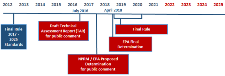
But after Donald Trump won the presidential election on November 8, 2016, the EPA ditched the MTE process it had obligated itself to follow in October 2012 and reconfirmed in July 2016. On November 30, the EPA proposed its final MTE and allowed the public only 30 days during the holiday season to comment on its 268-page proposal and 719-page technical support document. Despite receiving more than 100,000 comments, the EPA finalized the MTE only two weeks after the comment period closed, just in time to hand the incoming Trump administration a regulatory fait accompli.

Abandoning its regulatory commitments in this manner was arbitrary, capricious, and an abuse of discretion. Stakeholders did not have adequate time to prepare detailed technical comments on the proposal and TSD, and the agency did not have adequate time to review all significant comments. Worse, by finalizing its portion of the MTE 14 months in advance, the EPA disengaged from what was supposed to be coordinated review and concurrent rulemaking.

As the Alliance of Automobile Manufacturers observed, the EPA confronted NHTSA with two defective choices: either (1) produce an independent evaluation that “may be substantially different and not at all harmonized with EPA’s determination,” or (2) “align itself with EPA’s determination regardless of the existence of facts and analyses that would suggest the need for a different outcome.” Either way, “the process now bears no resemblance to the coordinated effort that was envisioned in the midterm evaluation.” The EPA made a mockery of the so-called harmonized national program.

President Trump in his first administration put the band back together. The Safer Affordable Fuel-Efficient (SAFE) Vehicles Rule, a joint rulemaking by NHTSA and the EPA, featured coordinated and consistent CAFE and tailpipe CO₂ standards.

However, under the Biden administration, the EPA again decoupled its regulatory activities from NHTSA’s. The two agencies proposed and finalized their rulemakings at different times rather than concurrently, and there was no effort to “harmonize” CAFE and tailpipe CO₂ standards. That was because the Environmental Policy and Conservation Act (EPCA), the nation’s fuel economy statute, prohibits NHTSA from making fuel economy standards so stringent that automakers must average in the “fuel economy” of zero-emission vehicles to comply (more on this later). Inconsistency was inevitable, because the Biden administration refused to let EPCA constrain the EPA’s climate ambition.

Moreover, the EPA is not the expert in setting fuel economy standards, but it is in effect setting fuel economy standards through its greenhouse gas vehicle standards. The EPA’s lack of comparative expertise in setting fuel economy standards and NHTSA’s unquestioned exclusive role and expertise on such standards is yet another factor showing the EPA’s greenhouse gas vehicle standards violate the major questions doctrine.

Congressional Decisions not to Regulate. An additional factor that informs the application of the major questions doctrine is whether Congress “conspicuously and repeatedly declined to enact [a regulatory program] itself.”  The majority in Massachusetts gave short shrift to the EPA invoking “postenactment congressional actions and deliberations it views as tantamount to a congressional command to refrain from regulating greenhouse gas emissions.”  The majority would be right to not take such actions as a “command” but such actions certainly are a relevant factor that helps to inform whether the major questions doctrine applies as explained in West Virginia.

It is helpful to first start with how Congress has in fact clarified that greenhouse gases are not to be regulated. The terms “greenhouse gas,” “greenhouse effect,” and “global warming” appear nowhere in the texts of the 1970 and 1977 Clean Air Act (CAA) amendments, which also contain no title, section, or subsection on global climate change. The Supreme Court’s implicit claim in Massachusetts v. EPA and explicit assertion in American Electric Power v. Connecticut that the 1970 CAA “speaks directly” to the question of the EPA’s regulatory authority with respect to carbon dioxide (CO₂) is unsupported by either clear textual evidence or basic legislative history.

The CAA did not address the issue of global climate change until the 1990 amendments, and then only obliquely. The 1990 CAA mentions “carbon dioxide”—but only once, in Section 103(g) of the CAA, a provision authorizing EPA to develop “nonregulatory strategies and technologies”  for reducing “multiple air pollutants … from stationary sources, including fossil-fuel power plants.”

Lest anyone miss the drift, the word “nonregulatory” occurs six times. And lest anyone draw regulatory inferences from carbon dioxide’s inclusion in a list of “air pollutants,” the provision concludes: “Nothing in this subsection shall be construed to authorize the imposition on any person of air pollution control requirements.”

Similarly, the 1990 CAA mentions “global warming” only once, in another nonregulatory provision, Section 602(e) of the CAA, which requires the EPA to “publish”—i.e., estimate—the “global warming potential” of ozone-depleting substances. A similar admonition immediately follows: “The preceding sentence shall not be construed to be the basis of any additional regulation under this title [i.e., the CAA].”

Such caveats were necessary to clarify what powers the 1990 CAA Amendments did not grant to the EPA, because climate policy had been a bone of contention in Congress’s deliberations on the amendments.

S. 1630, the Senate version of the 1990 CAA Amendments, introduced in 1989, contained a provision (section 206) to establish CO₂ emission standards for new motor vehicles. The Senate Environment and Public Works Committee approved a bill called “The Stratospheric Ozone and Climate Protection Act,” envisioned as Title VII of the amended CAA. Title VII would have authorized EPA to regulate ozone-depleting substances based in part on their “global warming potential.” It would also establish CO₂ and methane emissions reduction as a national goal.

The full Senate deleted the automobile CO₂ standards. House and Senate conferees subsequently discarded the other regulatory climate provisions. Instead of declaring a national goal to reduce CO₂ and methane emissions or authorizing regulation of ozone-depleting substances informed by their “global warming potential,” the conference committee, chaired by Sen. John Dingell (D-MI), approved CAA Sections 103(g) and 602(e). As noted, those provisions clearly instruct the EPA not to infer delegations of regulatory power. 

Subsequent efforts by members of Congress to enact GHG cap-and-trade legislation, national clean energy standards, or national ZEV mandates came to nought. Although “post-enactment congressional actions and deliberations” cannot repeal any authorities Congress previously delegated to the EPA, the failure of such bills after decades of climate advocacy provides significant support to show that Congress “conspicuously and repeatedly declined to enact [a regulatory program] itself.” This is yet another important reason why the major questions doctrine prohibits the regulation of greenhouse gas emissions from new motor vehicles.

III. Greenhouse Gas Vehicle Standards are Not Authorized Since the Relevant Emissions Do Not Cause or Contribute to Dangerous Air Pollution

It is helpful to restate the relevant language for analyzing whether greenhouse gas emissions cause or contribute to dangerous air pollution:

(1) The Administrator shall by regulation prescribe (and from time to time revise) in accordance with the provisions of this section, standards applicable to the emission of any air pollutant from any class or classes of new motor vehicles or new motor vehicle engines, which in his judgment cause, or contribute to, air pollution which may reasonably be anticipated to endanger public health or welfare.

New Motor Vehicles. The relevant emissions to be analyzed must first be properly identified.  As explained earlier in the comment, the relevant emissions must be from new motor vehicles, not existing ones. The 2009 endangerment finding looked to existing vehicles, not just new vehicles. This is problematic not merely because it violates the clear language of the statute, but also because the standards set pursuant to Section 202(a) are prospective in nature. They are connected to regulating cars going forward, not looking backwards. After all, the agency is not regulating existing vehicles under Section 202(a) so why would the emissions be based on vehicles that are irrelevant when establishing the standards? Further, as a practical matter and as explained in the Proposed Rule, using existing vehicle data is a problem because it increases the amount of emissions “because newer vehicles and engines tend to be more efficient and emit less.”

Class or Classes. The relevant emissions must be based on the emissions from “any class or classes,” not a combination of the emissions of every possible motor vehicle the agency can regulate under 202(a), from motorcycles, buses, to light-duty cars. Yet this is what the EPA did in the 2009 endangerment finding.

Separating the Endangerment Finding from Setting the Standards. In the Endangerment Finding, the EPA took the unreasonable step of analyzing “cause or contribute” and “endangerment” separately from the setting of standards. The EPA explained in the Endangerment Finding:

As discussed in the Proposed Findings, typically endangerment and cause or contribute findings have been proposed concurrently with proposed standards under various sections of the CAA, including CAA section 202(a). EPA received numerous comments on its decision to propose the endangerment and cause or contribute findings separate from any standards under CAA section 202(a)….

EPA, in this case, is fully prepared to go forward with the contribution and endangerment determination, while it is not ready to proceed with rulemaking for each and every category of new motor vehicles in the first rulemaking to set emissions standards.

This makes no sense. Section 202(a)(1) is not a mere academic exercise. It is a section on setting standards for any class or classes of new motor vehicles. The agency in the Endangerment Finding is arguing that it can do the analysis of Section 202(a)(1) regardless of what standards it sets, if any. By its logic, the agency could just do the analysis and not set any standards. It may not even have a desire to set standards at all but could just begin doing the analysis for the sake of it. This demonstrates the disconnect between the Endangerment Finding and any resulting standards.

The agency treats endangerment and the analysis in 202(a)(1) as a free pass that it can use whenever it has the inclination to regulate specific vehicles. The agency could keep that free pass for decades or forever, but what about timing concerns? The analysis and the standard setting should be simultaneous so that the standards are justified on and reflect current factors. Otherwise, by the time the EPA got around to setting a standard, the analysis could easily be outdated.

Further, the analysis required under Section 202(a) is only triggered when developing standards for a specific class or classes of vehicles. After all, the purpose of the analysis is to justify the regulation of the class or classes and to inform the standards.

The Proposed Rule is correct when it states:

As a result of this new conception of authority, the EPA may issue a single endangerment finding in the abstract with respect to emissions from all sources potentially subject to CAA section 202(a) (and their existing-source counterparts) without addressing the danger posed by any particular source category or the causal role of that particular source category in any identified danger….

We propose that Congress enacted CAA section 202(a) as an integrated regulatory provision for a reason, and that giving effect to the language of the statute requires the issuance of emission standards only when the Administrator has made an integrated finding of both endangerment and cause or contribution. Put another way, we propose that it is impermissible for the Administrator to make an endangerment finding without prescribing the emission standards required in response to such a finding,…

This common sense understanding of the statute is not new. As the EPA explains in the Proposed Rule, “This proposed interpretation is consistent with the EPA’s implementation of CAA section 202(a) and similar provisions of the CAA prior to 2009.”

Effect of the Emissions. In the Endangerment Finding, the EPA tried to come up with as big a number as possible for total emissions. Count emissions from existing vehicles, not just new vehicles. Check. Count all vehicles the agency can regulate under Section 202(a) as opposed to analyzing by class or classes. Check. Count foreign sources of vehicle emissions and not just domestic sources. Check.

The EPA determined that emissions from all Section 202(a) source categories accounted for 4.3 percent of global greenhouse gas emissions. This served as the basis for the EPA in the Endangerment Finding to conclude that these emissions “contribute to the air pollution that endangers public health and welfare.”

This 4.3 percentage is much higher than it should be because of how the agency determined the relevant emissions to be analyzed. If properly limited to emissions from new domestic vehicles or engines by class or classes, the number would be far lower. The Proposed Rule states “the best available data indicate that GHG emissions from light- and medium-duty vehicles in the United States amounted to approximately 1.8 percent of global GHG emissions in 2022.”  This may even be a high number (the full methodology is not clear to these authors), but it is less than 4.3 percent. At least it is based on domestic vehicles by class or classes.

The question of whether emissions “contribute” to dangerous air pollution does not mean there only has to be a contribution of a single molecule. Even the Endangerment Finding recognized that a de minimis contribution was likely insufficient.  It is true that unlike Section 111 of the Clean Air Act, the language does not say “contribute significantly.”  But there is a big gap between de minimis and significant. The appropriate contribution level lies within this gap.

Despite the very low number of 1.8 percent, the agency should not base the question of “contribution” solely on the volume of emissions. A volume-based threshold by itself does not inform whether there really is a proper contribution. Setting such a threshold is just an arbitrary process. Is 20 percent enough? Does five percent suffice?

As a practical matter, the EPA necessarily needs to look at what effect the emissions from new motor vehicles have on the dangerous air pollution. If such an analysis were not required, then how would the agency distinguish volume thresholds across pollutants? Maybe it makes sense for a lower or higher percentage to apply to the emissions of a greenhouse gas than to an actual air pollutant, but to figure that out, the agency would inherently need to look at the connection and effect of the emissions on the dangerous air pollution.

Also, if Congress simply wanted the agency to just come up with some volume threshold by itself, then why even direct such a request to the Administrator and leave it to his judgment? Such an arbitrary process hardly requires any expertise. The reason why the Administrator is expected to use his judgment under 202(a)(1) is to ascertain whether emissions of a specific pollutant make any difference to the dangerous air pollution and what level of these emissions make enough of a difference to say those emissions “contribute” to such pollution.

A volume threshold alone comparing domestic new motor vehicle emissions to total global emissions does not tell us whether those emissions make any difference to the “air pollution” or the danger it poses to public health or welfare. Under this volume approach, the EPA could claim a contribution even if the emissions do not have any detectable effect on the danger level of the air pollution. Given the purpose and language of the Clean Air Act and Section 202(a), which is to protect the public’s health or welfare from dangerous air pollution, not analyzing these effects is unreasonable.

If the emissions in no way (or in a de minimis way) affect the danger level from the air pollution, then it would be unreasonable to claim that the emissions contribute to the dangerous air pollution. This is all consistent with the Proposed Rule’s argument that “the emission must cause or contribute to the danger posed by the air pollution to a sufficient extent to satisfy the standard for regulation.”

So, how do we answer the question about the effect on danger levels?

The basic narrative explaining the potential dangers associated with the “atmospheric mix”—the global bucket of GHG “air pollution”—is well known. Rising atmospheric GHG concentration increases global temperatures, which may adversely affect weather patterns and sea levels, which may adversely affect public safety, property damage, labor productivity, GDP growth, energy costs, and other economic variables, which may adversely affect public health and welfare.

Since global warming is the first link in the chain of endangerment attributed to rising GHG concentration, the first step in determining whether GHG emissions from a class or classes of US new motor vehicles contribute to that danger is to calculate their effects on global warming.

In his comments on the Proposed Rule, American Enterprise Institute (AEI) economist Benjamin Zycher uses the US government’s standard climate-policy calculator, a model called MAGICC, to assess the potential contribution of new US motor vehicles to global warming. His analysis may be summarized as follows.

At the time of the Endangerment Finding, the EPA reported that US carbon dioxide-equivalent emissions in 2005 totaled 7,109 million tons or 18 percent of global annual emissions. If one assumes 3.0°C climate sensitivity, then achieving NetZero US emissions by 2050 would reduce global warming in 2100 by 0.137°C. Assuming former NASA scientist James Hansen’s standard deviation estimate of 0.11°C,  “the year 2100 temperature impact of U.S. net-zero GHG emissions would be either undetectable or barely detectable.” At the time, the EPA estimated that Section 202 vehicles accounted for 23.5 percent of total US GHG emissions. Thus under a simplifying assumption of linearity, achieving NetZero for Section 202 US motor vehicles would reduce year 2100 global temperatures by 0.032°C, “an outcome obviously not statistically significant and thus undetectable.”

But if the warming effects of US new motor vehicle GHG emissions are undetectably small, even more so are the putative second and third order effects of those emissions. Therefore, US new motor vehicle emissions do not “contribute” to dangerous air pollution pursuant to Section 202(a).

Finally, this discussion is consistent with the Proposed Rule’s discussion of causation and proximate cause:

Congress legislated against background legal principles, including principles of causation and proximate cause. These “default rules” are “presumed to have [been] incorporated, absent an indication to the contrary in the statute itself,” and nothing in the text of CAA section 202(a) indicates that Congress intended to depart from ordinary legal meaning. As a general matter, there is a point at which harm no longer has a sufficiently close connection to the relevant conduct to reasonably draw a causal link. We propose that emissions from new motor vehicles and new motor vehicle engines in the United States do not have a sufficiently close connection to the adverse impacts identified in the Endangerment Finding to fit within the legal meaning of “cause” or “contribute.” [Footnotes removed].  

IV. The Biden Administration’s De Facto EV Mandate Violates the Major Questions Doctrine

Our discussion of the major questions doctrine has already discussed many of the reasons why greenhouse gas vehicle standards under 202(a) are prohibited. This included some discussion of the Biden EPA’s de facto EV mandate. However, it is important to provide even more details on this specific rule and also to stress that regardless of what happens with the endangerment questions, this rule should be repealed.

In April 2024, the EPA set tailpipe CO₂ standards for MY 2027-2032 motor vehicles that aggressively squeeze gas- and diesel-powered passenger cars and light trucks out of the US automobile market. The standards function as de facto electric vehicle (EV) sales mandates, i.e. a ban on sales of gas- and diesel-powered cars and trucks.

By MY 2032, the projected market share of plug-in electric vehicles (PEVs), which include battery electric vehicles (BEVs) and plug-in hybrid electric vehicles (PHEVs), increases to 69 percent, while the projected market share of internal combustion (ICE) and hybrid (HEV) vehicles decreases to 31 percent.

As policy analyst Phil Kerpen pointed out, the EPA’s April 2024 rule is California’s gas-car ban with a two-year delay and the out-years hidden.

Note, the tailpipe CO₂ standards adopted by the EPA in December 2021 already required the incremental banning of ICE vehicle sales. The EPA acknowledged that its GHG emission standards for MY 2023-2026 vehicles “will necessitate greater implementation and pace of technology penetration through MY 2026 using existing GHG reduction technologies, including further deployment of BEV and PHEV technologies.” 

Specifically, the EPA estimated “the standards can be met with gradually increasing sales of plug-in electric vehicles in the U.S., from about 7 percent market share in MY 2023 (including both fully electric vehicles (EVs) and plug-in hybrid vehicles (PHEVs)) up to about 17 percent in MY 2026.”

Among other things, this means the Biden EPA’s de facto EV mandate rules use the same Clean Power Plan regulatory tactic the Court struck down in West Virginia v. EPA (2022). That tactic is to drive fossil-fuel technologies out of the marketplace by setting emission standards that are increasingly beyond their capacity to meet.

Like the Clean Power Plan, the Biden EPA’s vehicle electrification mandates are unlawful under the Court’s major questions doctrine. Many of the relevant arguments were brought up in the earlier section on major questions and greenhouse gas vehicle standards. But it is helpful to bring up some important points here as well.

As in the Clean Power Plan, the EPA sought to settle energy and climate policy issues Congress was still debating. The agency aimed once again to wield the powers of an industrial policy czar, “restructuring” the automotive sector with huge knock-on effects for the US oil, gas, and biofuel industries, as well as for the electric power sector. And it did so based on an unauthorized policy judgment, namely, that it would be “best” if fossil-fueled vehicles exit the marketplace. 

Private petitioners in Texas v. EPA concisely explain the unlawful pattern:

Just as in West Virginia, EPA is claiming the power to shift the Nation’s energy policy by reverse-engineering its preferred balance of technologies through emission standards. In West Virginia, it attempted to force a shift from coal-fired plants to wind- and solar-powered plants; here, it attempts to force a shift from liquid-fuel vehicles to electric vehicles.

V. Additional Arguments

1) The decoupling of NHTSA’s fuel economy scheme with EPA’s greenhouse gas vehicle standards provides a strong statutory basis for why Section 202(a) does not authorize greenhouse gas vehicle standards. NHTSA is responsible for fuel economy, but the EPA through its greenhouse gas vehicle regulations is usurping NHTSA’s role and rendering the CAFE program superfluous.   
  
2) EPCA § 32902(h) prohibits NHTSA from considering the “fuel economy” of “dedicated vehicles,” such as EVs, when prescribing fleet-average fuel economy standards. In other words, NHTSA is prohibited from making CAFE standards so stringent that automakers cannot comply unless they average in the “fuel economy” of vehicles that do not run on liquid fuels. Yet the EPA, which is not authorized to regulate fuel economy in the first place and is not the agency charged with this responsibility, is not only usurping NHTSA’s job but also doing so in a way that NHTSA itself is prohibited from doing (taking EVs into account). This is a statutory basis for prohibiting, at a minimum, the EPA from considering EVs when setting greenhouse gas vehicle standards.  

3) Battery-electric vehicles are not a class of new motor vehicles nor do they belong in any class under Section 202(a). This section of the Clean Air Act applies to new motor vehicles that emit air pollutants, which does not include these EVs.

4) Vehicle standards in general, if based on fleet averaging, should be prohibited. The Biden de facto EV mandate, like all previous tailpipe GHG standards, are fleet-average standards. The Court in Massachusetts is partly to blame because it told the EPA to “avoid inconsistency” with NHTSA’s CAFE standards, which are fleet-average standards. Additionally, the EPA has been setting fleet-average standards for criteria pollutants since the 1980s, at the behest of automakers.

In Texas v. EPA, private petitioners argue that fleetwide-average emission standards are unlawful under CAA § 202(a).  The Clean Air Act “unambiguously precludes fleetwide-average emission standards under Section 202(a).” To begin with, Section 202(a) “says nothing about averaging across fleets.”  Moreover, fleetwide averaging clashes with “the design and structure of [Title II] as a whole.”  “Title II sets forth a comprehensive, interlocking scheme for enforcing emission standards through testing, certification, warranties, remediation, and penalties. Fleetwide-average standards are incompatible with these provisions, which are ‘designed to apply to’ individual vehicles and ‘cannot rationally be extended’ to fleets. Id. at 322.”  

Section 202(a) is explicitly linked to Section 202(b), which “sets forth specific light-duty vehicle emission standards that EPA must promulgate in ‘regulations under’ Section 202(a).” Such standards, which are required for carbon monoxide, hydrocarbons, and oxides of nitrogen, “necessarily apply to vehicles individually, not to fleets on average.”  For example: “The regulations under subsection (a) of this section applicable to emissions of oxides of nitrogen from light-duty vehicles and engines manufactured during model years 1977 through 1980 shall contain standards which provide that such emissions from such vehicles and engines may not exceed 2.0 grams per vehicle mile.”  There is no room in such language for averaging. Congress did not intend to allow automakers to produce some vehicles that emit more than the standard provided other vehicles emit less.

Section 202(b) testing requirements confirm that those standards apply to individual vehicles, petitioners contend: “In particular, EPA must ‘test any emission control system incorporated in a motor vehicle or motor vehicle engine . . . to determine whether such system enables such vehicle or engine to conform to the standards required to be prescribed under [Section 202(b) of the Act].”  If the system complies, EPA must issue a ”verification of compliance with emission standards for such system.”  

Section 205 of the Clean Air Act states that any violation “shall constitute a separate offense with respect to each motor vehicle or motor vehicle engine,” with each offense subject to its own civil penalty of up to $25,000.  How do you impose a penalty that is a “separate offense with respect to each motor vehicle or motor vehicle engine” when doing a fleet wide average?

Petitioners draw the only reasonable conclusion: “Those requirements plainly contemplate standards that apply to individual vehicles and their emission-control systems. Not only does the statutory text frame the inquiry as whether an individual ‘vehicle’ or ‘engine’ conforms to the emission standards, but the provision’s foundational premise—that an emission-control system can enable a vehicle to meet emission standards—depends on individually applied standards.”  

VI. Climate Science/Greenhouse Gas Vehicle Standards are Not Authorized Since the Air Pollution May Not Reasonably Be Anticipated to Endanger Public Health or Welfare 

This section chiefly address topic area C—2, “The scientific underpinnings of the Endangerment Finding are weaker than previously believed and contradicted by empirical data, peer-reviewed studies, and scientific developments since 2009.” This section is also responsive to C—1, which requests comment on “scientific developments that are being subject to public comment for the first time,” C—23, which requests comment on the “quality, objectivity, utility, and integrity of information” disseminated by the Fifth National Climate Assessment (NCA5) and, as indicated, previous NCAs,  and C—27, which requests comment on “aspects of the Endangerment Finding that may have fallen short of the administrative law requirement that agency action be reasonable and reasonably explained.”

The EPA’s 2009 Greenhouse Gas Endangerment Finding (hereafter, “Endangerment Finding”) lists the “major assessments” by the U.S. Global Change Research Program (GCRP)/Climate Change Science Program (CCSP),  Intergovernmental Panel on Climate Change (IPCC), and the National Research Council (NRC) as the “primary scientific basis supporting the Administrator’s endangerment finding.”  The Endangerment Finding’s Technical Support Document (TSD) says much the same but gives pride of place to the IPCC, which had published its Fourth Assessment Report (AR4) two years earlier, in 2007.  Our comments examine key scientific assumptions of the Endangerment Finding, its TSD, AR4, and later “major assessments” often touted as updating and vindicating the Endangerment Finding.

Our Basic Findings and Approach

Mainstream climate research has a scientific integrity problem due to its reliance on a triply biased methodology. For decades, the usual practice has been to run overheated models with inflated emission scenarios and ignore or belittle humanity’s remarkable capacity for adaptation. That approach is wired to exaggerate the physical impacts of greenhouse gas emissions and the harmfulness of such impacts. All three biases compromise the assessment reports underpinning the Endangerment Finding.

What that means is that the EPA should have no confidence in the validity of the Endangerment Finding. Indeed, given mankind’s adaptive capabilities, we may reasonably anticipate the continuation of the long-established decline in climate-related mortality and in relative economic impact of extreme weather, especially in societies that protect economic liberty and welcome energy abundance. In other words, endangerment of public health and welfare from carbon dioxide (CO₂)-related “air pollution” is not reasonably anticipated.

In a sense, almost all our comments on scientific issues respond to C—27, which asks whether the Endangerment Determination flouts standards of reasonable action and explanation. It does flout such standards because the Endangerment Determination is built on the triply biased methodology mentioned above. Moreover, the biases were not clearly communicated by the authors.

To make our case, we often present the information in reverse chronological order. Just as it took decades to develop the scientific “consensus” on which the Endangerment Finding relies,  it also took years to discover and document the flaws of the “consensus” approach. That is due in part to transparency deficits in consensus climatology that impeded independent review.  Moreover, in a science projecting changes in climate metrics over decades to centuries, significant divergences between original hypotheses and observations may take considerable time to clearly emerge.

Accordingly, in the sections that follow, documentation of consensus climatology’s reliance on overheated models, inflated emission scenarios, and unreasonably pessimistic adaptation assumptions begins by reviewing patterns of bias in recent official assessment reports—the IPCC’s Fifth and Sixth Assessment Reports, published in 2013 and 2021, and the USGCRP’s Fourth and Fifth NCAs, published in 2018 and 2023. Those reports are often invoked as updating and validating the Endangerment Finding. Having clarified the biases in the later assessment reports, we document the same distortions in the Endangerment Finding’s scientific basis. 

Overheated Models

To project the physical impacts of climate change, the IPCC, USGCRP, and other “mainstream” researchers run general circulation models (GCMs) and earth system models (ESMs) with various emission scenarios. The IPCC works with climate modeling groups around the world to produce and evaluate the models used in its assessment reports. This exercise is called the Coupled Model Intercomparison Project (CMIP). There have been six CMIPs, the first one in 1996. The CMIP3 model ensemble was used in the IPCC’s 2007 Fourth Assessment Report (AR4), the CMIP5 ensemble in the IPCC’s 2013 Fifth Assessment Report (AR5) and NCA4, and CMIP6 ensemble in the IPCC’s 2021 Sixth Assessment Report (AR6) and NCA5.

CMIP models make projections about the evolution of global annual average temperatures out to the year 2100 and beyond. There is no way to directly test the accuracy of those projections. However, the models can hindcast global temperature changes in the past, and those projections can be compared to observations. That is what atmospheric scientist John Christy and colleagues have done in a series of studies over the past two decades.

The chart below shows the mean and spread of CMIP5 model projections in the tropical mid-troposphere compared to the averages of three independent empirical datasets: satellites, balloons, and re-analyses. Compared to the observations, the models on average project more than twice the tropical bulk atmosphere warming during 1979-2016. 

Source: Christy (2017). Solid red line—average of all the CMIP5 climate models; thin colored lines—individual CMIP-5 models; solid figures—weather balloon, satellite, and reanalysis data for the tropical troposphere.

The next chart shows that only one CMIP5 model, the Russian INM-CM4, accurately tracks temperature change through the depth of the tropical troposphere. 

Source: Christy and McNider (2017). Tropical atmosphere temperate trends from 25 CMIP5 models compared to four radiosonde (weather balloon) datasets.

The superior accuracy of INM-CM4 likely has something to do with its climate sensitivity estimate, which is the lowest of any CMIP5 model. Climate sensitivity is customarily defined as the amount of warming that occurs after the climate system fully adjusts to a doubling of carbon dioxide-equivalent (CO₂e) greenhouse gas concentration. INM-CM4 has a climate sensitivity of 1.8°C. In contrast, GFDL-CM3, which has a sensitivity of 4.8°C, projects a warming trend that is literally off the chart. 

One might suppose the new and improved CMIP6 models used in AR6 would be more accurate. Not so—instead, they are worse. On average, CMIP6 models hindcast about 2.3 times the warming rate measured by satellites and weather balloons not only in the tropical troposphere but also in the global troposphere. Warming rates in all CMIP6 models are higher than the observed trend, in most cases significantly so.

Source: Adapted from McKitrick and Christy (2020). Red bars are CMIP6 temperature projections. White dashed line is the average of observations. Black dashed line is the model average projection.

Readers may wonder why the comparisons either focus on the tropical troposphere or highlight it. After all, nobody lives there!

The tropical mid-troposphere is uniquely suited for testing the validity of climate models. That is because: (1) Nearly all models predict strong positive feedbacks (accelerated warming) in the tropical mid-troposphere; (2) the region is well-monitored by satellites and weather balloons; (3) the mid-troposphere is too distant from the surface to be influenced by urban heat islands; and (4) the models were not previously “tuned” to match the historical climatology in that region, hence are genuinely independent of the data used to test them.

That last point is the most critical. Modelers try to make their models realistic by adjusting climate parameters until hindcasts match historical temperature changes. For example, a modeler may adjust a GCM’s climate sensitivity estimate to keep it within an “acceptable range.” However, hindcasting data already used to calibrate a model is like peeking at the answers before taking a quiz. The only real way to test a climate model’s predictive skill (other than waiting 30+ years to see how things evolve) is to compare the model’s hindcasts to data that have not already been used to train the model. In other words, the model must be applied to data that are “out of sample.” That is Christy’s procedure. The results speak for themselves. The models are not realistic. They run too hot.

A reasonable explanation is that even when tuned to keep climate sensitivity within an “acceptable range,” the models still overestimate climate sensitivity. One might suppose that after the mismatch between the CMIP5 models and observations, the CMIP6 models would have lower climate sensitivity estimates. Instead, about 35 percent of CMIP6 models have climate sensitivities higher than the warmest CMIP5 model.

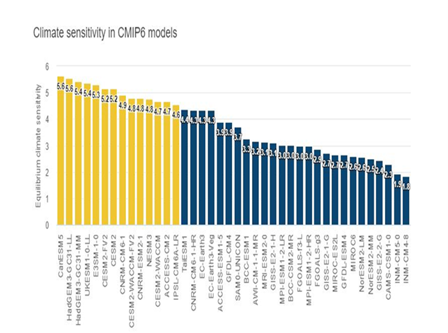
Source: Hausfather (2020). Yellow bars show CMIP6 models with higher sensitivity than any CMIP5 model. Blue bars show CMIP6 model sensitivities within the CMIP5 range.

Zhu et al. (2020) exposed the surrealism of the high-sensitivity CMIP6 models. They ran the CESM2 model, which has a sensitivity of 5.2°C, with an emission scenario in which CO₂ concentrations reach 855 parts per million (ppm) by 2100. The model produced a global mean temperature “5.5°C greater than the upper end of proxy temperature estimates for the Early Eocene Climate Optimum.” That was a period when CO₂ concentrations of 1,000 to 2,000 ppm persisted for millions of years. Moreover, the CESM2 tropical land temperature exceeds 55°C, “which is much higher than the temperature tolerance of plant photosynthesis and is inconsistent with fossil evidence of an Eocene Neotropical rainforest.” 

The authors conclude: “Our study illustrates that the development and tuning of models to reproduce the instrumental record does not ensure that they will perform realistically at high CO₂.” More colloquially, tuning models to match historical climatology does not ensure they have predictive skill.

How did the IPCC cope with the “hot model problem” reported by Zhu et al. and other investigators? In previous IPCC reports, Hausfather et al. (2022) explain, the IPCC “simply used the mean and spread of models to estimate impacts and their uncertainties”—a method dubbed “model democracy” because each model counted equally in the overall assessment. In AR6, the IPCC decided to apply weights to the models before averaging them. 

While “weighting” avoids the embarrassment of treating all projections, even the most outlandish, as equally credible, it does not correct the basic methodological flaw—a reliance on persistently errant models.

That is not what meteorologists do. They do not base weather forecasts on the average and spread of all models regardless of their track records. Rather, they use the model or models shown by experience to have predictive skill for specific types of weather in specific regions.

One might wonder whether climate models are more accurate when, like weather models, they assess changes at regional scales. They are not. For example, all 36 CMIP6 models overshoot the 12-state US Corn Belt 1973-2024 summer temperature trend, with 30 models exceeding observations by factors of 2 to 8.

Source: Spencer 2025, Climate Modeling and Reality

We therefore concur with the Proposed Rule’s assessment that “models relied upon by the Endangerment Finding may be incorrect with regard to warming in the U.S. Corn Belt given the divergence of recent empirical data from projected trends.”

The CMIP5 and CMIP6 model ensembles are the most critical inputs to the AR5, AR6, NCA4, and NCA5 assessment reports that supposedly update and vindicate the Endangerment Finding. At a minimum, the epic failure of models touted as more advanced than the CMIP3 models used in AR4 means that a key scientific basis for the Endangerment Finding is weaker today, not stronger.

But what of the Endangerment Finding itself—did warming projections and observations significantly diverge even then, and did the Endangerment Finding TSD acknowledge the models’ lack of realism? The answer to the first question is yes, as the chart below shows. The answer to the second is no.

Source: John Christy

In the 2000s, it was still difficult to obtain tropospheric temperature projections from climate modelers. Christy, however, was able to obtain surface temperature projections from the models and then compare those with the HadCRUT surface record  and with satellite data adjusted to match surface temperatures. In the chart above, temperature trends start in the year indicated on the X-axis and end in 2009. The observations (squares) all fall much below the AR4 model average (diamonds), usually about half the magnitude of the modeled trend.

The Endangerment Finding TSD correctly reports that mid-tropospheric temperatures since 1979 as measured by satellites are warming at a “flat” (non-accelerating) rate of 0.11°C to 0.15°C/decade in US government satellite research, and 0.12°C to 0.19°C/decade in AR4 —rates consistent with modest warming (~2.0°C) by century’s end. However, there is no information comparable to Christy’s analysis in the chart above.

Instead, what we find elsewhere in the TSD is the claim that models are realistic because they can reproduce 20^th century global-scale changes in surface temperature, but only if the models are run with “both natural and anthropogenic forcings.” The TSD illustrates that assessment with the chart below.

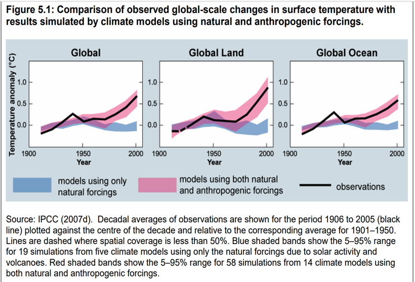
As the chart shows, the claim that models are realistic when run with both natural forcings and anthropogenic GHGs comes from AR4.

The IPCC’s reasoning looks suspiciously circular. AR4 assumes the models’ understanding of natural “forcings” is accurate enough to account for all significant natural variability operating through the 20^th century. That assumption is contradicted by the ongoing debate over the causes of early 20^th century global warming (1910-1940) and the US Dust Bowl.  If, instead, the IPCC underestimates natural variability, then the models of course would not work without the addition of GHG forcing.

Moreover, as noted above, because models are trained (“tuned”) to simulate 20^th century land and ocean temperatures, a model’s ability to reproduce “in sample” data is no assurance of predictive skill.

Christy may have been the first to challenge AR4’s claim that model projections match observations when the models include both natural and anthropogenic forcings. However, he had to wait until AR5 provided a chart of natural and anthropogenic forcings in the tropical troposphere. Even then, the data required for model testing had to be inferred from an online supplement. When Christy enlarged and clarified the chart, he discovered that model projections and observations almost entirely diverge unless the models are run with natural variability alone.

Source: John Christy, Annotated version of IPCC AR5 Figure 10.8(b), vertical warming pattern for tropics (20S to 20N). Horizontal axis: °C/decade.

We therefore concur with the Proposed Rule’s assessment that “recent data and analyses suggest that attributing adverse impacts from climate change to anthropogenic emissions in a reliable manner is more difficult than previously believed and demand additional analysis of the role of natural factors and other anthropogenic factors such as urbanization and localized population growth.”

As indicated, unrealistically high climate sensitivity estimates appear to be an important factor in the persistent mismatch between model projections and observations. In AR4, the IPCC’s “best estimate” of climate sensitivity was 3°C.  The average sensitivity in 24 empirically constrained studies  published during 2011-2018 is 2.0°C.

Source: Patrick J. Michaels and Ryan Maue, March 6, 2019. The median (indicated by the small vertical line) and 90% confidence range (indicated by the horizontal line with arrowheads) of the Roe-Baker ECS distribution is indicated by the top black arrowed line. The median value in Row-Baker is 3°C. The ECS mean of the 24 studies is 2°C.

In a series of cases dealing with the EPA’s modeling of air pollutant risks, the D.C. Circuit Court of Appeals has repeatedly held that an agency’s use of a model is “arbitrary” if the model bears “no rational relationship to the reality it purports to represent.” Climate models that repeatedly overshoot observations may be useful for various academic purposes but are unfit to inform endangerment determinations and other regulatory decisions imposing large costs and risks on fundamental sectors of the economy. Logically, the same verdict should apply to unrealistic emission scenarios and adaptation assumptions.

Inflated Emission Scenarios

The IPCC, USGCRP, and other government actors typically run the CMIP ensembles with prominent emission scenarios that expressly or tacitly assume the world returns to a coal-dominated energy system over the course of the 21^st century.

Although the Shale Revolution began in 2007, many scenarists assumed until quite recently that learning-by-extraction and economies of scale would make coal the increasingly affordable backstop energy for the global economy. For example, some analysts assumed oil and gas would become increasingly costly to extract, creating sizeable markets for coal-to-liquid fuels and coal gasification.

The IPCC and USGCRP have been the main legitimizers of the two most influential scenarios used in recent climate impact assessments—RCP8.5 and SSP5-8.5. RCP8.5 is the high-end emission scenario in the AR5, NCA4, and the IPCC’s 2018 Special Report on Global Warming of 1.5°C.  SSP5-8.5 is the high-end emission scenario in AR6 and NCA5.

Although neither scenario was originally designed to be the baseline or business-as-usual scenario, both have been widely misrepresented—including by the USGCRP and IPCC—as official forecasts of where 21^st century emissions are headed. 

RCP8.5 tacitly assumes global coal consumption increases almost tenfold during 2000-2100. See the chart on the next page.

Source: Riahi et al. (2011).

Nothing like that is happening or expected to happen. For example, in RCP8.5, global coal consumption roughly doubles during 2020-2050. In contrast, in the Energy Information Administration’s (EIA’s) most recent International Energy Outlook, global coal consumption during 2022-2050 increases by 19 percent in the high economic growth case and declines by 13 percent in the low economic growth case. 

The increasing affordability of natural gas and the plethora of policies mandating and subsidizing renewables invalidate RCP8.5 as a business-as-usual emission scenario, but so do coal industry economics. Coal producer prices more than doubled during 2000-2010 and are now about 3.5 times higher than in 2000. 

Unsurprisingly, in the International Energy Agency’s (IEA) baseline emission scenarios (“pledged policies,” “current policies”), global CO₂ emissions in 2050 are about half those projected by SSP5-8.5.

Source: Hausfather and Peters (2020)

In 2022, Resources for the Future (RFF) published updated baseline emission scenarios, informed by IEA and other market forecasts. In the RFF’s baseline projection, global CO₂ emissions are about half those projected in SSP5-8.5 in 2050 and less than one-fifth those projected in 2100. The EPA adopted the RFF baselines as the best available for its November 2023 report on the social cost of greenhouse gases.  

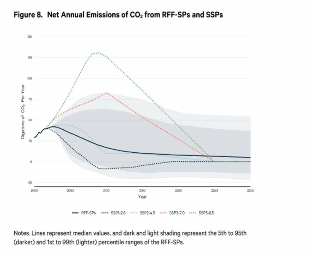
Source: Kevin Rennert et al. (2022). The solid black line is the RFF’s baseline projection. The dotted green line is SSP5-8.5.

For perspective, in NCA4, RCP8.5 was the business-as-usual scenario and RCP4.5 was the climate change mitigation policy scenario. RCP4.5 was estimated to reduce harmful climate change impacts on labor productivity, extreme heat mortality, and coastal property by 48 percent, 58 percent, and 22 percent respectively. The new RFF baseline closely aligns with SSP2-4.5, which has the same radiative forcing as RCP4.5. Among other things, that means GHG emissions cause or contribute significantly less to dangerous air pollution than the IPCC and USGCRP estimated in their post-AR4 reports.

However, the RFF baseline may already be out of date. Recent information suggests that the most realistic emission scenario is not SSP2-4.5 but an even “cooler” scenario, SSP2-3.4. In other words, the current global emissions trajectory adds 3.4 W/m² of warming pressure by 2100. Assuming 3°C climate sensitivity, SSP2-3.4 results in 2.0°C-2.4°C of warming by 2100. Keep in mind that lower sensitivities find support in recent research.  

It is difficult to overstate the distorting influence RCP8.5 and SSP5-8.5 have had on climate research and public discourse. Google Scholar lists 51,900 papers on RCP8.5 and 15,500 on SSP5-8.5. Cursory sampling suggests that very few studies challenge the plausibility of those scenarios. Of the first 50 entries for both RCP8.5 and SSP5-8.5, only one is critical—Hausfather and Peters (2020) cited above. All others are studies that use RCP8.5 or SSP5-8.5 to project climate change impacts.

In AR6, the IPCC finally acknowledged the “low” likelihood of RCP8.5 and SSP5-8, citing “recent developments in the energy sector” and the IEA’s baseline emission scenarios. However, the extreme scenarios continue to dominate, with RCP8.5 and SSP5-8.5 receiving 41.5 percent of scenario mentions. When combined with another unrealistic high-end scenario, SSP3-7.0 (the orange dotted line in the RFF figure above), total mentions of extreme scenarios in AR6 rise above 50 percent. 

Like AR6, NCA5, published in November 2023, also runs the CMPI6 model ensemble with the SSP emission scenarios. However, unlike AR6, NCA5 declines to determine that SSP5-8.5 is “no longer plausible without a reversal” of current energy market trends.  Instead, NCA5 contends all the scenarios are “plausible futures.”   That is plainly false.

NCA4 contains a worse breach of scientific integrity, which is relevant to the EPA’s reconsideration, because it shows how easily the combination of overheated models and inflated emission scenarios can be manipulated to frighten the public.

Perhaps the only thing anyone not directly involved in producing NCA4 will remember about it is its dire warning that unchecked warming could raise end-of-century global temperatures by 8.0°C, cutting US GDP by 10 percent. The New York Times duly reported that “finding” as the report’s big takeaway. 

Those estimates came from a single study, Hsiang et al. (2017).  The authors ran the warm-biased CMIP5 model ensemble with three AR5 RCPs, including the warm-biased RCP8.5. NCA4 reproduced Hsiang et al.’s chart projecting GDP loss as a function of global-mean temperature.

However, NCA4 did not reproduce Hsiang et al.’s chart showing the probabilities of those temperature increases. The chart below shows that even when CMIP5 is run with RCP8.5, global warming hits 8.0°C in only 1% of model runs. In the IPCC’s likelihood scale, anything with a 0-1% probability is deemed “exceptionally unlikely.”

Source: Hsiang et al. (2017). An 8°C warming has a probability of 0.01 when CMIP5 is run with RCP8.5.

NCA4 concealed from readers the extreme unlikelihood of its worst-case scenario, allowing The New York Times and other media to present an implausible disaster as a probable future absent new stronger commitments to ‘global action.’

Turning now to AR4 and the USGCRP reports informing the EPA’s 2009 Endangerment Finding, we find the same reliance on implausible emission scenarios.

American Enterprise Institute (AEI) scholar Roger Pielke, Jr. recently posted the relevant information on his blog. As he explains, the Endangerment Finding relied on two sets of scenarios to project future changes in climate and the associated risks: the six scenarios developed in the IPCC’s Special Report on Emission Scenarios (SRES, 2000) and three Climate Change Science Program (CCSP) scenarios.

To facilitate comparison with later IPCC and USGCRP reports, Pielke, Jr. presents two charts showing the nine scenarios and their radiative forcings:

---

The left panel shows the six SRES scenarios (along with three earlier IPCC scenarios, the IS92 scenarios) in terms of 2100 radiative forcing. The right panel shows the three CCSP scenarios and their projected radiative forcings to 2100.

Pielke renames the scenarios for their 2100 W/m² radiative forcings and lists them from highest to lowest forcing:

1. A1FI-9.2 (SRES)
2. IGSM-8.6 (CCSP)
3. A2-8.1 (SRES)
4. MERGE-6.6 (CCSP)
5. MiniCAM-6.4 (CCSP)
6. A1B-6.1 (SRES)
7. B2-5.7 (SRES)
8. A1T-5.1 (SRES)
9. B1-4.2 (SRES)

He observes:

• The nine scenarios “are heavily skewed to very high levels of 2100 radiative forcing, with two even more extreme than RCP8.5.”
• Eight of the nine “project a central estimate” of 3.0°C above pre-industrial temperature by 2100, “a value today viewed to be unlikely.”
• The average radiative forcing across all nine scenarios is 6.7 W/m² (which is well above the IEA baseline scenarios).
• Of the nine scenarios, only B1-4.2 “is consistent with what today are called ‘current policy’ scenarios.”

Pielke, Jr. further points out that each of the three CCSP scenarios “project that coal will be the primary source of energy in the US and the world.” He comments: “No one believes that anymore.”

Here are the CCSP energy market projections. In each of the six panels, coal without carbon capture—depicted by the purple segments—is either the dominant component of the US and global energy mix or the largest single component:

Like the later IPCC and USGCRP reports, the Endangerment Finding relied on unrealistic and warm-biased models and emission scenarios.

Ignore or Depreciate Adaptation

Arguably the worst analytic error of the Endangerment Finding was its decision to exclude adaptation from the analysis of endangerment. The EPA judged that adaptation is a “potential response” to endangerment and thus outside the scope of the agency’s analysis. Being a “response,” adaptation “presupposes” endangerment, hence does not reduce it.

That argument overlooks important differences between physical, chemical, biological, or radioactive substances that directly endanger public health or welfare via inhalation, dermal contact, or other routes of exposure, and CO₂. Carbon dioxide is non-toxic to humans and animals at any concentrations projected to occur from fossil fuel combustion, does not affect visibility, and is an essential building block of plant life (hence also of the planetary food chain). Equally important, in contrast to other airborne substances that pose direct threats to human health and welfare, the risks from CO₂ emissions come from potential changes in weather and sea levels over periods of decades to centuries.

The EPA’s argument would be solid if applied to soot and smog, hazardous air pollutants, or radioactive fallout. When making an endangerment determination about such substances, it would be preposterous to consider the availability of gas masks, hazmat suits, or medical treatments for radiation exposure. However, it is equally preposterous to exclude adaptation when considering potential changes in weather and sea levels over decades to centuries. Adapting to varied and even extreme environmental conditions is what human beings have been doing since time immemorial. And it works!  

Several big-picture trends indicative of increasing climate resilience and safety are never mentioned in the Endangerment Finding and other official assessments of climate change impacts and risks:

• Over the past 70 years, which is roughly the modern warming period, humanity achieved unprecedented improvements in global life expectancy, per capita income, and per capita food supply.

• US and global corn, wheat, and rice yields (tons per hectare) increased decade by decade since the 1960s. Combined global corn, wheat, rice, and soybean output doubled since 1980.

• Globally, the decadal annual average number of people dying from climate related disasters declined from about 485,000 per year in the 1920s to about 14,000 per year in the past decade—a 97 percent reduction in annual climate-related mortality.

• Factoring in the fourfold increase in global population since the 1920s, the average person’s risk of dying from extreme weather has decreased by 99.4 percent.

• Taking an even longer view, global deaths from extreme weather are conservatively estimated at 50 million in the 1870s. That frightful weather-related death toll declined to an estimated 5 million in the 1920s, 500,000 in the 1970s, and 50,000 in the 2020s. Global weather-related deaths in the first half of 2025 totaled about 2,200—very likely the lowest weather-related mortality of any six-month period in recorded history.

• Warmth can accelerate mosquito breeding cycles and expand mosquito habitat. Nonetheless, from 2000 to 2020, global incidence of malaria (number of new cases per 1,000 population at risk) declined by 27.5 percent while global deaths from malaria declined by 30 percent.

• The number of excessive heat days in U.S. cities increased since 2010. However, U.S. heat related mortality was lower in 2010-2018 than in any previous eight-year period since 1975.
• Globally, climate-related economic losses have increased as population and exposed wealth have increased. However, losses as a percentage of exposed wealth declined almost five-fold from 1980-1989 to 2007-2016, with most of that progress occurring in low-to-middle income countries.
• Similarly, although the number of US “billion-dollar disasters” is increasing (due to increases in population and exposed wealth), US annual average weather-related losses as a share of GDP declined from slightly over 0.2 percent in 1990 to somewhat below 0.2 percent in 2019.

Although not reflected in the Endangerment Finding, the EPA has documented the superior cost-effectiveness of adaptation in reducing endangerment. The EPA’s May 2017 climate change sectoral analysis, a technical report for NCA4, estimates that cumulative coastal property damage through 2100 will total $3.6 trillion under RCP8.5 and $3.508 trillion under RCP4.5. In other words, reducing RCP8.5 emissions to RCP4.5 levels decreases cumulative coastal property damages by $92 billion or 2.6 percent. In contrast, proactive adaptation decreases RCP8.5 costal property damages to $820 billion—a 77.2 percent reduction. Moreover, mitigating emissions to RCP4.5 levels reduces coastal property damages by only $20 billion or 0.5 percent beyond the protection provided by adaptation alone. The contribution from mitigation is so small it is barely discernible in the EPA’s chart.

Adaptation’s power to reduce or even avert endangerment may be even greater than the EPA’s 2017 sectoral analysis implies. In his book False Alarm, Bjorn Lomborg reviews Hinkel et al. (2014), a sea-level rise study published in Proceedings of the National Academy of Sciences.  The study includes a worst-case scenario in which sea-levels driven by high-end RCP8.5 warming flood up to 350 million people every year by century’s end, with costs reaching $100 trillion or 11 percent of global GDP annually.

However, those extraordinary damages are projected to occur only if people do nothing more than maintain current flood control infrastructure. If “enhanced” adaptive measures are taken, so that coastal protections keep pace with sea-level rise, annual flood costs increase from $11 billion in 2000 to $38 billion in 2100. Similarly, annual dike costs increase from $13 billion to $48 billion. However, Lomborg notes, “the total cost to the economy will actually decline, from 0.05 percent of GDP to 0.008 percent.” Moreover, the number of people experiencing flood damage drops from 3.4 million in 2000 to 15,000 in 2100—a 99.6 percent reduction in flood victims.

In other words, with forward-looking adaptation, Hinkel et al. project that sea-level rise from extreme warming can be much less damaging to people and the global economy in 2100 than current sea levels are today. To exclude this type of analysis from an endangerment determination is a form of cherry-picking. It is neither rational analysis nor reasoned decision making (C—27). 

We therefore concur with the Proposed Rule’s assessment that “lack of analysis of adaptation generally, and particularly with respect to sea level rise, reduces confidence in the reasonableness, accuracy, and reliability of the assumptions and conclusions in the Endangerment Finding.”

We also concur that the Endangerment Finding “did not adequately balance the projected adverse impacts attributed to global climate change with the potential benefits” of rising CO₂ concentration, which “advances public health and welfare by directly impacting plant growth and therefore the price and availability of food, the success of American agricultural and related industries, and the traditional capacity of the United States to export significant food supplies around the world for economic and humanitarian purposes.”

Summing Up the Science Discussion The scientific assessments informing the Endangerment Finding, like those that came later and were cited in support of it, reflect three fundamental biases—a preference for overly sensitive models, increasingly implausible emission scenarios, and unreasonable depreciation of human adaptive capabilities.

Consequently, the EPA should have no confidence in the conclusion that CO₂ emissions from new motor vehicles cause or contribute to air pollution which may reasonably be anticipated to endanger public health or welfare. On the contrary, societies that protect economic liberty and welcome abundant energy may reasonably anticipate a future of increasing climate safety and diminishing relative impact of climate related economic damage.

Conclusion

Greenhouse gas regulation is not typical regulation. It gives the EPA the ability to reshape major portions of the economy and change the way Americans live their lives. This is a critical reason why the EPA should carefully assess whether it does have such sweeping authority.

There are numerous questions before the agency, most of which are legal in nature and look far different than they would have right after Massachusetts v. EPA. Significant developments have occurred including the fleshing out of the major questions doctrine. There are also numerous problems with the 2009 endangerment finding based both on scientific grounds and the improper application of Section 202(a) of the Clean Air Act, such as improperly determining whether emissions from new motor vehicles contribute to dangerous air pollution.   

We urge the agency to finalize a rule that concludes greenhouse gas vehicle standards are unauthorized under Section 202(a) of the Clean Air Act.
 

Sincerely,

Daren Bakst
Director, Center for Energy and Environment and Senior Fellow
Competitive Enterprise Institute

Marlo Lewis
Senior Fellow, Center for Energy and Environment
Competitive Enterprise Institute

Click below to read full comments.