The Scientific Case for Vacating the EPA’s Carbon Dioxide Endangerment Finding

Executive Summary
The U.S. Environmental Protection Agency’s (EPA) 2009 “Endangerment Finding” from carbon dioxide (CO2) and other greenhouse gases grants the agency a legal mandate that can have profound and far-reaching effects. The Finding is based largely on a Technical Support Document that relies heavily upon other mandated reports, the so-called National Assessments of global climate change impacts on the United States.
The extant Assessments at the time of the Endangerment Finding suffered from serious flaws. We document that using the climate models for the first Assessment, from 2000, provided less quantitative guidance than tables of random numbers—and that the chief scientist for that work knew of this problem.
All prospective climate impacts in the Endangerment Finding are generated by computer models that, with one exception, made systematic and dramatic errors over the climatically critical tropics. Best scientific practice would be to emphasize the working model, which has less warming in it than all of the others.
Instead, the EPA relied upon a community of wrong models.
New research compares what has been observed to what is forecast, and finds that warming in this cen- tury will be modest—near the lowest extreme of the prospective range given by the United Nations.
The previous administration justified its policy choices by calculating the Social Cost of Carbon [dioxide]. We interfaced their model with climate forecasts consistent with the observed history and enhanced the “fertilization” effect of increasing atmospheric concentrations of CO2. We find that making the warming and the vegetation response more consistent with real-world observations yields a negative cost under almost all modeled circumstances.
This constellation of unreliable models, poor scientific practice, and exaggerated estimates of the Social Cost of Carbon argue consistently and cogently for the EPA to reopen and then vacate its endangerment finding from carbon dioxide and other greenhouse gases.
Introduction
The Environmental Protection Agency’s (EPA) 2009 “Endangerment Finding” is the basis for comprehensive regulations of carbon dioxide emissions under the Clean Air Act.1 It is based on another EPA report called a Technical Support Document (TSD), which, as this paper will show, is seriously flawed because it is based upon climate models that are making large systematic errors. Therefore, the subsequent impact models based on them are also unreliable. These project, among other things, changes in crop yields, ecosystems, and social systems caused by changes in climate. Further, the EPA did not follow best scientific practices in determining either the course of future climate or the cost of current and future carbon dioxide emissions.
Subsequent to the Endangerment Finding, the Obama administration justified its interventionist policies with its calculation of a figure known as the Social Cost of Carbon (SCC). The SCC is a monetary estimate of the damages supposedly caused by an incremental ton of carbon dioxide (CO2), the principal contributor to human-induced climate change, emitted in a given year. Discernible in neither economic nor meteorological data, social cost values are guesstimates produced by computer programs called “integrated assessment models” (IAMs). What IAMs “integrate” is a speculative model of how carbon dioxide emissions will change the climate with a speculative model of how climate change will affect consumption, GDP, and health. Only one of these models, known as FUND (for Framework for Uncertainty, Negotiation, and Distribution), contains an explicit term to account for the fertilization effects of increasing atmospheric carbon dioxide. All of the IAMs are based upon a warming that is too great—in which sensitivity to carbon dioxide is too high—based upon recently observed data.
Here, we will see that more realistic values for climate sensitivity and the fertilization effect of carbon dioxide, along with realistic discount rates, can produce a SCC that is negative, or something that could be considered a net benefit, certainly calling the concept of “endangerment” into question.
We will show that multiple and internally consistent lines of evidence, such as an inability to define serious costs with realistic model parameters, and two tragic flaws in the supporting “science summary” documents that underpin the original finding, should compel the EPA to reconsider and then vacate its 2009 Endangerment Finding.
History of the Endangerment Finding
The Endangerment Finding was produced in response to a 2007 Supreme Court decision, Massachusetts v. EPA, that the Clean Air Act of 1970 empowered the EPA to regulate emissions of carbon dioxide, if the agency found that they endangered human health and welfare.
The case against the EPA was originally brought by 12 states and several environmental advocacy organizations. It eventually came before the District of Columbia appellate court, which upheld an original decision in favor of the EPA’s choice not to regulate CO2, on the grounds of scientific uncertainty as to the amount and effects of climate change actually caused by increasing atmospheric concentrations.
The appellate court decision was split 2-1, with a vigorous dissenting opinion by Judge David S. Tatel. The Supreme Court granted a writ of Certiorari to Massachusetts v. EPA on June 26, 2006. Judge Tatel’s dissent was highly influential when the case came before the Court, argued on November 29, 2006. The decision, a narrow 5-4 verdict, was announced on April 2, 2007. The majority held that the Clean Air Act did grant the EPA authority to regulate greenhouse gas emissions as “air pollutants.”
The timing was late in President George W. Bush’s second term, which deferred substantive action. Incoming President Barack Obama did not, placing global warming as his second highest priority in his first inaugural address (behind national health care). His EPA issued a preliminary “finding of endangerment” less than three months later, on April 17, 2009, and a final finding was announced on December 7, 2009.2 That date coincided with the opening of the 15th Conference of the Parties to the United Nations 1992 Framework Convention on Climate Change (UNFCCC), also known as the Rio Climate Treaty. The 2009 meeting was supposed to adopt a new emissions reduction protocol to replace the failed 1997 Kyoto Protocol, but it failed to do so.
The Endangerment Finding is backed by a Technical Support Document, which itself was largely based on the Fourth Assessment Report (AR4) of global warming by the United Nations Intergovernmental Panel on Climate Change (IPCC)3 and the second National Assessment of climate change impacts on the United States by the U.S. Global Change Research Program (USGCRP).4
Both of the foundational documents for the TSD have only one method to predict future climate—a large series of computer simulations of global climate with enhanced greenhouse gases, known as general circulation models (GCMs) or Earth system models (ESMs). The output of these models is then used to drive “impact” models, which apply to the many aspects of life, projecting changes in migration, death, nutrition, mental illness, among others.
If the GCM/ESMs can be shown to be fatally flawed, then their prospective climate forecasts are useless. Therefore, any forecasts of changed impacts are worse then useless; they may even have negative utility, because impact models have their own error terms and those interact multiplicatively with the errors in the GCM/ESMs. The application of this error cascade to policy can provoke unneeded suffering and impose grotesque and gargantuan opportunity costs. In this eventuality, the Endangerment Finding becomes an exercise in expensive rhetoric.
Are The National Assessments Tainted?
The final version of the Technical Support Document, published on December 7, 2009, relied heavily upon a document published by the U.S Global Change Research Program, “Global Climate Change Impacts in the United States”, also known as the Second National Assessment (NA-2) report. Since then, it has become clear that the models used for prospective climate in that report made significant systematic errors in the three-dimensional tropical atmosphere with significant implications concerning the reliability of subsequent forecasts for temperature and precipitation over large expanses of the planet.
The first National Assessment (NA-1) was published in 2000. Thomas Karl, Director of the National Oceanic and Atmospheric Administration’s (NOAA) National Climatic Data Center (NCDC), Jerry Melilo of the Marine Biological Laboratory, and Thomas R. Peterson, also of NCDC led the National Assessment Synthesis Team (NAST). Like the subsequent NA-2, it had a fatal flaw.
The design of the NA-1 was similar to the succeeding Assessments. All future impacts were generated from the output of general circulation climate models. At the time NA-1 was under development, NAST had eight GCMs to choose from to describe 21st century climate. They chose two: a) the Canadian Climate Centre model, which produced the greatest temperature changes over the U.S. of all eight, and b) the model from the U.K. Hadley Center, a part of the Meteorological Office, which produced the largest precipitation changes.
In our peer review of the draft NA-1, my then-colleague Chip Knappenberger and I looked at how well those two models could do the simplest of tasks—simulating 10-year running means of coterminous U.S. temperature averages over the 20th century, such as, for example, 1900-1909, 1901-1910, and so on. They could not do it. The answers the models gave were worse than simply assuming the 20th century average value. In other words, the models added errors to the raw data. What they did was ex- actly analogous to a student taking a four-option multiple choice test and getting less than 25 percent correct. The NA-1 models actually supplied “negative knowledge”. You knew less about 20th century U.S. climate by using them.
I emailed Karl my result, as we were on good professional terms. He responded that indeed we were correct and that further, the models exhibited the same failure on running means of one, five, 10 (which we analyzed), 20, and 25 years. Using climate models that do not work to assess the effects of climate change (with subsequent policy recommendations) is a scientific malpractice.5 (Karl and Melilo were also on the team that assembled NA-2, along with Anthony Janetos of the environmental advocacy group World Resources Institute. NA-2 also had systematic problems.)
— Patrick Michaels
Systemic Flaws in the Second National Assessment
The 2009 Second National Assessment of climate change impacts in the United States (NA-2) is the principal U.S-specific reference in the Technical Support Document for the Endanger- ment Finding. The weakness of NA-2 was apparent in its draft form. As one of these authors (Michaels) and Chip Knappenberger noted in public comments submitted on behalf of the Cato Institute:
Of all of the “consensus” government or intergovernmental documents of this genre that [we] have reviewed in [our] 30+ years in this profession, there is no doubt that this is the absolute worst of all. Virtually every sentence can be contested or does not represent a complete survey of a relevant literature.
There is an overwhelming amount of misleading material in the CCSP’s [Climate Change Science Program’s] “Global Climate Change Impacts in the United States.” It is immediately obvious that the intent of the report is not to provide an accurate scientific assessment of the current and future impacts of climate change in the United States, but to confuse the reader by a loose handling of normal climate events (made seemingly more frequent, intense, and damaging simply by our growing population) presented as climate change events. Additionally, there is absolutely no effort made by the CCSP authors to include any dissenting opinion to their declarative statements, despite the peer-reviewed literature being full of legitimate and applicable reports that provide contrasting findings. Yet, quite brazenly, the CCSP authors claim to provide its readers—“U.S. policymakers and citizens” with the “best available science.” This proclamation is simply false.
The uniformed reader (i.e., the public, reporters, and policy-makers) upon reading this report will be [led] to believe that a terrible disaster is soon to befall the United States from human- induced climate change and that almost all of the impacts will be negative and devastating. Of course, if the purpose here is really not to produce an unbiased review of the impact of climate change on the United States, but a political document that will give cover for EPA’s decision to regulate carbon dioxide, then there is really no reason to go through the ruse of gathering comments from scientists knowledgeable about the issues, as the only science that is relevant is selected work that fits the au- thors’ preexisting paradigm.6
In 2012 we published an addendum in the form of a palimpsest that featured a point-by-point rebuttal of specific faulty statements in the NA-2.7 For example, under “Key Finding” #7, NA-2 says:
7. Risks to human health will increase. Harmful health impacts are related to increasing heat stress, waterborne diseases, poor air quality, extreme weather events, and diseases transmitted by insects and rodents. Reduced cold stress provides some benefits. Robust public health infrastructure can reduce the potential for negative impacts. (p.89)8
Our addendum notes:
7. Life expectancy and wealth are likely to continue to increase. There is little relationship between climate and life expectancy and wealth. Even under the most dire climate scenarios, people will be much healthier and wealthier in the year 2100 than they are today. (pp. 139-45, 158-61)9
We urge readers interested in documenting the problems between NA-2 and the endangerment finding to do their own side-by side comparisons of both NA-2 and our response, shown in Appendix 1.
Despite all of the problems noted above, the Endangerment Finding was declared final on December 7, 2009. The next section looks at some critical findings subsequent to its publication, which will be important to any attempt to vacate it.
GCM Model Evaluation: Extant Models from the Time of the Endangerment Finding
The Technical Support Document for the Endangerment Finding relies on the climate models in the IPCC’s Fourth Scientific Assessment. (AR4). Certain behaviors of these models underscore the weakness of the scientific justification for the Endangerment Finding.
It has been known since the 19th century that the temperature response to a given increment of a greenhouse gas such as carbon dioxide is logarithmic, which means that it decreases with succeeding increments of emissions. Global atmospheric data, directly taken at Mauna Loa, Hawaii, beginning in 1958, and subsequently from other remote monitoring locations such as in Alaska and Antarctica, reveal a slow exponential growth in atmospheric concentration (see Figure 1).
In climate models, the combination of a logarithmic response and an exponential concentration increase can produce a near-linear rise in temperature with time, which is the case for the AR4 models. Furthermore, observed temperature change in recent decades resembles the linear changes in the AR4 models. Figure 2 shows global average temperatures from the Climate Research Unit at the University of East Anglia that were available at the time of the TSD and the endangerment finding. Despite the nascent warming “pause” that can be seen developing in the early 21st century, a first-order linear fit of the observations is highly significant and any second-order single curve fit adds no more power to the analysis.
Figure 1. Atmospheric carbon dioxide concentration at Mauna Loa, Hawaii, has been increasing as a very low-order exponential function since regular monitoring began in 1958.
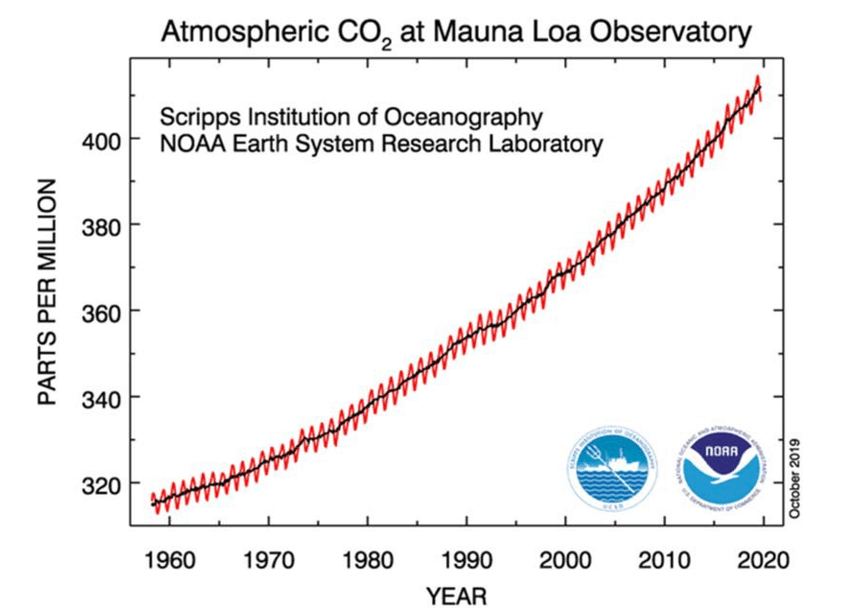
Source: University of California San Diego Scripps Institute of Oceanography/National Oceanic and Atmospheric Administration.
The linearity of the warming that began in 1977 allows one to discriminate between the AR4 models that serve as the basis for prospective forecasts in the TSD, which is shown in Figure 3. The result is that the best-fit warming lies at the low end of the AR4 projections. The 21st-century rise is 1C, which is consistent with subsequent “low sensitivity” estimates.10
GCM/ECM Model Evaluation: The Next Generation of Models after the Endangerment Finding The IPCC’s Fifth Assessment Report (AR5) was published in 2013 and contained a new suite of models, including updates of some of the AR4 models.
John Christy of the University of Alabama-Huntsville has uncovered some troubling systematic behavior of these models over the Earth’s tropics.
Figure 2. Global temperature anomalies, 1977-2008 (the year before the endangerment finding)
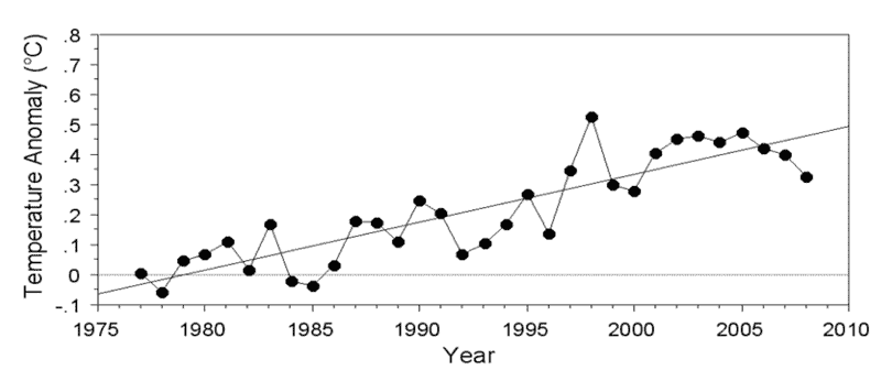
Source: Climate Research Unit, University of East Anglia, data downloaded in 2009 (2008 was the last year for which there was complete data prior to the 2009 endangerment finding). The starting year, 1977, marks the initiation of the second warming period of the 20th century; the first was from 1910 to 1945.
Figure 3. AR4 climate models (thin colored lines), average of the AR4 models (dark black dots), 1977-2008 observed global average surface temperature (red dots), and (solid red line) the linear trend of surface temperature when the 1977 temperature and the mean model temperature are set equal.
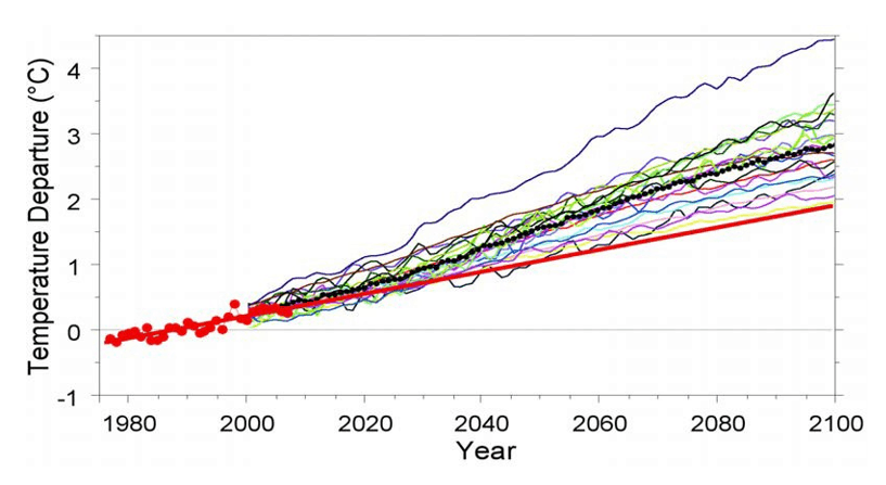
Data from the Climate Research Unit, University of East Anglia, from the iteration that was available in 2009.
Understanding the future behavior of the tropical troposphere (the lower atmosphere) is crucial to any confident assessment of potentially serious effects of climate change. That region is the source of moisture for the vast majority of rain storms that fall over midlatitude agricultural regions of North America and Europe, some of the most productive on Earth, including over 90 percent of the rain that falls over U.S. farmland in the growing season.11
Christy compared the output of all of the IPCC’s available models to temperatures averaged over the lower troposphere and warming rates predicted at different altitudes by those models. He studied those in the Fifth Assessment Report, which were supposed improvements over those in AR4. His study covered the Earth’s tropics (20oN-20oS), which cover over 37 percent of the planet’s surface.
With one exception, the AR5 models failed miserably. Figure 4 shows the average behavior of the models com- pared to three independent sets of observations:
-
Temperatures sensed by satellites;
-
Data from twice-daily launched weather balloons; and
-
The relatively new “reanalysis” data that infills data gaps with a physical model rather than extrapolation or statistical techniques.
|
Climate Sensitivity In climate science, “sensitivity” is the amount of warming projected by a climate model for a given change in the concentration of carbon dioxide. By comparing sensitivities, one can estimate different future warming regimes. The most commonly used sensitivity is called the “equilibrium climate sensitivity” (ECS). It is the amount of warming that is ultimately predicted by a given climate model for a doubling of the concentration of carbon dioxide over its preindustrial background concentration, nominally given as 280 parts per million (ppm). It is a purely theoretical number, because at the point that carbon dioxide attains the doubled concentration of 560 ppm, the concentration is still likely to continue to go up—that is, it will not be at “equilibrium”—but it provides a useful metric to compare modeling projections. Of more use is the “transient climate sensitivity” (TCS), which is the temperature change above the background (usually called the “preindustrial” temperature) that is modelled at the time that carbon dioxide doubles. This is a real number that should be observed in the second half of this century. As a general rule (though not in all cases), the forecast warming around the year 2100 is very close to the ECS, because after a nominal doubling around 2070, it would take around 30 years for most of the residual warming to be realized. |
The significance of a systematic model failure is profound. These models are the only basis for future projections in both the Endangerment Finding and its Technical Support Document. The fact that these are a generation beyond those used in the original finding demonstrates how poorly founded it was. This failure alone is a sufficient scientific reason to vacate the Endangerment Finding.
Instead of looking at the average temperature in the mid-troposphere, Figure 5 looks at individual levels from the surface to the bottom of the stratosphere.12 Note that all the models predict what is often called the “upper tropospheric hot spot” between
40,000 and 15,000 Pa (a measure of atmospheric pressure that corresponds, on average, to a layer between 23,000 and 45,000 feet above sea level), an area with a substantially enhanced warming rate compared to layers above and beneath it. The observed data (circles and squares) indicate that the models are predicting around three times the warming rate that is being observed.
Therefore, the models, as a community, predict a substantial and rapid warming in the “hot spot” layer that is barely occurring in reality.13 As noted earlier, getting the vertical distribution of temperature wrong renders some of the most important consequent forecasts wrong—such as those for precipitation over the world’s major agricultural regions.
Systemic errors in precipitation forecasting also render subsequent temperature forecasts questionable. Over a moist surface, the vast majority of incoming solar radiation is partitioned toward the evaporation of water rather than toward a direct heating of that surface. The ascent of moisture aloft in the tropics is proportional to the difference in temperature between the surface and the upper layers—the greater the difference, the more buoyant is the surface air, resulting in increased vertical transport of moisture. But if the input of moisture forecast is not reliable because of the vertical errors in the tropical data, then average forecasts of precipitation are similarly unreliable. The consequences for any endangerment finding are obvious: Therefore, there are no reliable models for future food production, which are based upon temperature and precipitation.
In Figures 4 and 5, close inspection will reveal that there is one model that comes reasonably close to what has been observed. It is the model from the Russian Institute for Numerical Mathematics, designated INM-CM4 in the Figures. Its ECS is 2.05oC, by far the lowest of all the models in the AR5 suite.15 Ironically, it is the accuracy of this model that points toward another fatal flaw in the Endangerment Finding.
Figure 4. AR5 climate models versus observations for the tropical mid-troposphere, 1979-2017
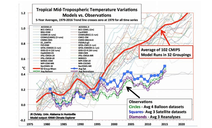
Solid red: AR5 model average; thin colored: individual model groupings; large colored lines: observations, including weather balloons, satellites, and reanalysis data. The plots begins in 1979 because that is when satellites began to return data.
Figure 5. Tropical pressure-level decadal temperature trends, 1979-2015
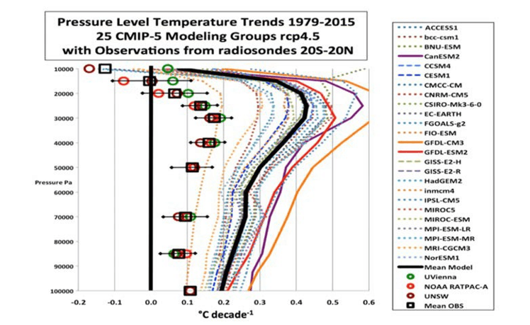
Solid black line: average for 25 model groups; thin colored lines: individual model groups; circles/squares: observed temperature trends from four different compilations.
Scientific Best Practice and the Endangerment Finding
In operational weather forecasting, forecasters do not simply average up all available models; rather, they tend to utilize the output of a model or a subset of models that has been shown to perform best in a given situation. For example, the model from the European Center for Medium Range Weather Forecasting (ECMWF) is often thought to be superior to the U.S. Global Forecast System (GFS) model with regard to hurricanes along the east coast of the United States. The ECMWF famously predicted the landfall, strength, and evolution of Superstorm Sandy in 2012 some eight days in advance. Had forecasters simply averaged all the various models together, they would have made a costly error and predicted Sandy would stay at sea.
The same should apply to forecasting climate change. Instead of using the best-performing model, the relevant National Assessments of climate change impacts on the U.S. use the distribution of model behavior in modeling the future. The last two iterations of these reports, in 2014 and 2018, would no doubt be used in any defense of a contested Endangerment Finding.
Here is how critical this practice is.
If the EPA endangerment finding followed the best scientific practice of emphasizing a model or models with particular expertise, the Endangerment Finding itself would be in danger.
That is because the one working model in Figures 4 and 5—the Russian INM-CM4—has the least 21st century warming of all the models in the AR5 suite and the lowest ECS, at 2.05oC.16 It also projects only 1.4oC of warming for this century. Both of these figures are far below the mean of all of the other AR5 models.17 Put simply, the one working model predicts only modest warming that would hardly warrant an endangerment finding. In addition, its new iteration for the upcoming Sixth Assessment report of the IPCC, INM-CM4.8 lowers the ECS to 1.83oC, far smaller than the other models, and very similar to what is in Lewis and Curry in their ECS calculation, which is discussed in the next section.
Consideration of the Social Cost of Carbon Dioxide
The Endangerment Finding finds further justification in the Obama administration’s calculations of what it called the “social cost of carbon [dioxide]” (SCC). It was determined by Interagency Working Groups that are tasked with running various “integrated assessment models.”18 Out of three available, only one,
the Framework for Uncertainty, Negotiation, and Distribution (FUND), contains an agricultural enhancement term that incorporates the “fertilization” effects of increasing atmospheric carbon dioxide. Because of this feature, we will concentrate on FUND.
With regard to future climate, the Administration used an ECS of 3.0oC and an outdated distribution around that mean published by Gerard Roe and Marcia Baker of the University of Washington in 2007.19 Their result are shown in the left-hand column in Table 1.
In recent years, sufficiently long observational data on ocean heat content and refined—reduced— estimates of the amount of cooling exerted by anthropogenerated sulfate aerosol emissions allow calculation of the ECS using reality-based energy balance models (rather than GCMs making serious errors). The many scientific publications using variations on this theme generally produce ECS values at or below the low limit of the distribution of the AR4 or AR5 models. This should not be surprising given Figures 2 and 3, which essentially integrate observations and model output.
Consequently, we calculated the SCC using the 2018 model calculation from Nicholas Lewis and Judith Curry, which has a sensitivity of 1.6o.20 The results are in the second column on the left in Table 1. It is obvious that this more realistic (and lower) sensitivity dramatically drops the SCC. Using a 5 percent discount rate, as shown in the table, the cost is currently slightly negative, which would imply a slight net benefit from emissions.
The agricultural enhancement term in FUND is based upon a literature that is generally a quarter-century old.
Since that period, much progress has been made in understanding agricultural fertilization and planetary greening from increased CO2. As a result, we increased the agricultural production component by 15 percent and 30 percent, respectively. These are shown in the two right hand columns of Table I. In seven out of eight cases, the SCC is negative, including all the 2050 calculations, with the exception of the 3 percent discount rate.
Table 1. Social Cost of Carbon using the FUND model with two discount rates
($2007 $/metric ton of CO2)
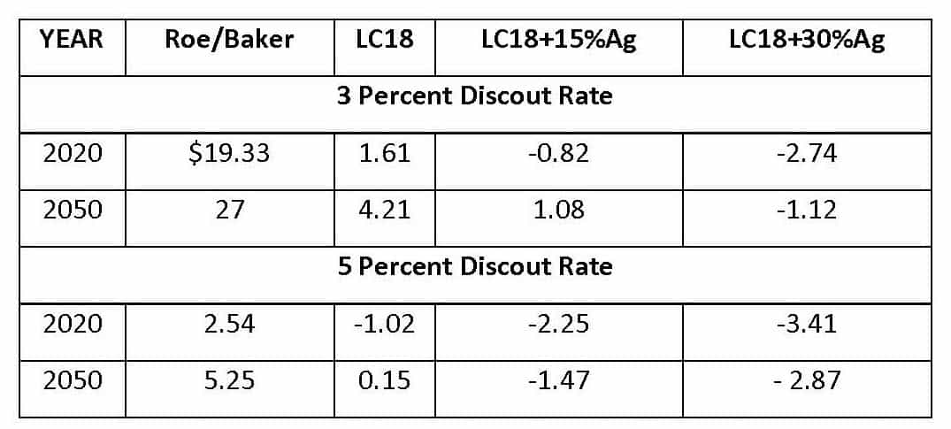
Left column: using the outdated Roe-Baker ECS distribution. Next column: Using the Lewis and Curry (2018) ECS distribution. Next column, same, but with a 15 percent enhancement of the agricultural term. Right column: Same but with a 30 percent agricultural enhancement.
As shown in Table 1, the SCC also varies with the assumed discount rate. We use both 3 percent and 5 percent, as did the Obama administration. While the Office of Management and Budget recommends using a 7 percent rate— the historical equity investment return average since 1900—the administration did not do so. Close inspection of Table 1 reveals a possible reason why. It appears, at the higher discount rate, even the Obama Administration’s SCC would have become negative even with the outdated Roe and Baker warming distribution.21
Rationale for the increased agricultural enhancement parameter
The agricultural enhancement terms in the FUND model are largely based upon references from the early 1990s that did not include advancements in carbon dioxide enrichment field experiments and remote sensing of increases in planetary greenness. For example, rice yields are not enhanced in FUND because of insufficient knowledge at the time. Yet, rice is the most important food grain on Earth.
It is now known that rice yields respond strongly to increased carbon dioxide. Hybrid rice shows a yield response of around 34 percent. In a 2016 review of the enhancement literature, the noted agronomist Bruce Kimball found that:
[T]he most exciting and important advances in regard to CO2 enrichment are the large yield responses of hybrid rice. … [T]he findings are indeed encouraging for the prospects of breeding rice varieties that can respond with higher grain yields at the elevated CO2 concentrations expected in the future.22
In his conclusion, Kimball notes that “many more [enhancement] experiments should be done to genetically screen and select for high responses to elevated CO2 of many genotypes of many major crops.23
Here, Kimball is implying that the passive yield enhancements implicit in FUND are underestimates because of the importance of both traditional genetic breeding and genetic engineering. There will be major efforts among breeders to incorporate genetics that display enhanced responses to both carbon dioxide and temperature.24
Also ignored in FUND is that temperature and carbon dioxide increases can act synergistically. Research published after Kimball’s comprehensive review shows this. In a laboratory study of soybeans it was demonstrated that elevated temperature increased soybean yields by 30 percent, elevated carbon dioxide by 51 percent, and, when combined (which must occur in the real world of the future), the increase was 65 percent.25
Satellite-recorded changes in global greening provide additional compelling evidence that future carbon dioxide fertilization is substantially underestimated in the social cost of carbon as estimated by FUND.
A 2016 study by research team led by Zaichun Zhu of Peking University, covering 1982 to 2009, found that the global ratio of greening to browning land was 9:1. Further, it found that nearly 90 percent of the greening is a result of human activity. Using a factor analysis, this study found that 70 percent of the greening was due to the increase in CO2, 9 percent from nitrogen deposition, 8 percent from climate change (mainly from lengthening growing seasons) and 4 percent from land use changes. All of these are from human activity.26
While the study by Zhu and colleagues was of a global nature, with no differentiation between agricultural and otherwise vegetated land, a 2019 paper by researchers from Beijing Normal University and the University of Maryland reported that agriculture- related trends were more than double those for the background “natural” vegetation.27
This clearly corroborates a 2018 study by French researchers that found breathtaking increases in agricultural greening. Along with natural vegetation, it analyzed greening in three agricultural strata: grassland, summer crops, and winter crops. By far, grassland covered more of the Earth’s surface than the other types of agriculture. The study, led by Simon Munier of the University of Toulouse, covered 17 years (ending in 2015) and found a remarkable 5 percent per year increase in grassland leaf area index (greening), which translated into 85 percent over the study period.28 Given that this is a true measure of potential yield increase, as grasslands are directly consumed by grazers, this is observed value several times the yield increases incorporated in the FUND model used to calculate the SCC. It is likely that our 15 percent and 30 percent additional enhancements are underestimates.
All of these findings indicate that the agricultural enhancement in FUND is too small. Our results shatter much of the SCC’s legitimacy in justifying the Endangerment Finding. Furthermore, as we note in our recent study, the majority of analogous calculated SCC values are negative, implying that, at least for much of this century, increasing atmospheric carbon dioxide confers a net benefit.29
Further Rationale for a Decreased Equilibrium Climate Sensitivity
Some additional guidance on the relevance of this to the Endangerment Finding can be seen in Figure 1 from a 2017 Norwegian study, led by Cecilie Mauritzen of the Norwegian Institute for Water Research, presented as Figure 6 here.30 Given the behavior shown in Figures 4 and 5, it seems logical that the lines with the least warming, given the three concentration pathways are model INM-CM4. Note that in each scenario, 21st century warming is at (RCP 8.5) or below (RCP 2.5 and 4.5) 1.5oC in the model that behaves the best in Figures 4 and 5.31 But RCP 8.5 is almost certainly an overestimate of 2100 radiative forcing because it does not properly account for the shift from coal to natural gas for electrical generation—now observed in the U.S., and, given supply and environmental considerations, likely to be adopted by China.32
Therefore, this projected temperature range is far below the 2.0oC goal of the Paris Climate Accord, and, given the inappropriateness of RCP 8.5, below even its 1.5o aspirational thresh- old. The INM-CM4 warming, which is the projection that should be used based upon best scientific practice, simply does not justify an endanger- ment finding.
Figure 6. Mean surface temperatures projected by the CMIP-5 models
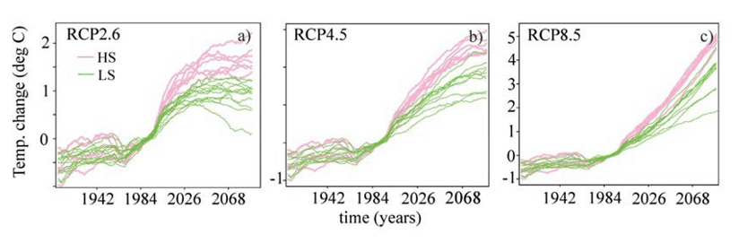
Figures are departures from the 1971-1999 average. The lowest line in each image is the Russian model INM-CM4, the one that best tracks temperature in the tropical troposphere.
Conclusion
The EPA’s 2009 Finding of Endangerment from carbon dioxide and other greenhouse gases is based upon a Technical Support Document that substantially relies on the 2009 National Assessment of climate change impacts on the U.S., published by the U.S. Global Change Research Program. The two extant National Assessments at the time of the Endangerment Finding publication were highly flawed. The first one engaged in extremely dubious science and the second one so cherry-picked the climate issue that it provided material for an entire point-by-point rebuttal—which in fact contained more scientific references than the USGCRP document. In Appendix 1, we excerpt the key findings in both the original and its palimpsest to show how radically different conclusions can be reached with regard to climate change impacts on the U.S. We have provided consistent evidence that future warming is likely to be at the lowest end of the 2007 suite of climate models that populated the EPA’s Technical Support Document, and that the next suite of models, in 2013, systematically overpredicted, by several times, the observed climate warming rate aloft in the tropical atmosphere. This is a critical error that largely invalidates forecasts of future precipitation, and therefore projections of agricultural impact.
After defining the important “sensitivity” of climate, we demonstrate that in the current suite of IPCC models, from 2013, that only one out of 102 model runs correctly simulates the tropical troposphere. Scientific best practice would be for forecasters to rely heavily upon this model and to heavily discount the rest. This model, the Russian INM-CM4, has the lowest sensitivity of all, which alone should compel EPA to vacate its 2009 endangerment finding.
We then show that previous federal calculations of the Social Cost of Carbon [dioxide] are greatly influenced by whether or not they include recent low-sensitivity estimates that are based upon refined knowledge of the cooling effects of sulfate aerosols.
They are also influenced by increasing the well-documented growth- and yield-enhancing effects of additional atmospheric carbon dioxide, based upon recent research. We cited extensive literature from recent years that now implies that the growth enhancement factor used in standard models is far too low, and raising it turns the SCC negative for much of this century. This, coupled with a demonstration that the mean sensitivity of the IPCC models is too high when compared to real-world climate and warming data, provides another compelling argument to vacate the EPA’s Endangerment Finding.
In summary, multiple and internally consistent lines of evidence compel the EPA to reconsider and then vacate its 2009 Endangerment Finding.
APPENDIX I
Key Findings from NA-2 and Compared to the “Addendum”. NA-2:
- Global warming is unequivocal and primarily human-induced. Global temperature has increased over the past 50 years. This observed increase is due primarily to human-induced emissions of heat- trapping gases. (p. 13)
- Climate changes are underway in the United States and are projected to grow. Climate-related changes are already observed in the United States and its coastal waters. These include increases in heavy downpours, rising temperature and sea level, rapidly retreating glaciers, thawing permafrost, lengthening growing seasons, lengthening ice-free seasons in the ocean and on lakes and rivers, earlier snowmelt, and alterations in river flows. These changes are projected to grow. (p. 27)
- Widespread climate-related impacts are occurring now and are expected to increase. Climate changes are already affecting water, energy, transportation, agriculture, ecosystems, and health. These impacts are different from region to region and will grow under projected climate change. (pp. 41-106,
107-152)
- Climate change will stress water resources. Water is an issue in every region, but the nature of the
potential impacts varies. Drought, related to reduced precipitation, increased evaporation, and increased water loss from plants, is an important issue in many regions, especially in the West. Floods and water quality problems are likely to be amplified by climate change in most regions. Declines in mountain snowpack are important in the West and Alaska where snowpack provides vital natural water storage. (pp. 41, 129, 135, 139)
- Crop and livestock production will be increasingly challenged. Many crops show positive responses to elevated carbon dioxide and low levels of warming, but higher levels of warming often negatively affect growth and yields. Increased pests, water stress, diseases, and weather extremes will pose adaptation challenges for crop and livestock production. (p. 71)
- Coastal areas are at increasing risk from sea-level rise and storm surge. Sea-level rise and storm surge place many U.S. coastal areas at increasing risk of erosion and flooding, especially along the Atlantic and Gulf Coasts, Pacific Islands, and parts of Alaska. Energy and transportation infrastructure and other property in coastal areas are very likely to be adversely affected. (pp. 111, 139, 145, 149)
- Risks to human health will increase. Harmful health impacts of climate change are related to increasing heat stress, waterborne diseases, poor air quality, extreme weather events, and diseases transmitted by insects and rodents. Reduced cold stress provides some benefits. Robust public health infrastructure can reduce the potential for negative impacts. (p. 89)
- Climate change will interact with many social and environmental stresses. Climate change will combine with pollution, population growth, overuse of resources, urbanization, and other social, economic, and environmental stresses to create larger impacts than from any of these factors alone. (p. 99)
- Thresholds will be crossed, leading to large changes in climate and ecosystems. There are a variety of thresholds in the climate system and ecosystems. These thresholds determine, for example, the presence of sea ice and permafrost, and the survival of species, from fish to insect pests, with implications for society. With further climate change, the crossing of additional thresholds is expected. (pp. 76, 82, 115, 137, 142)
- Future climate change and its impacts depend on choices made today. The amount and rate of future climate change depend primarily on current and future human-caused emissions of heat-trapping gases and airborne particles. Responses involve reducing emissions to limit future warming, and adapting to the changes that are unavoidable.
(pp. 25, 29)
Palimpsest
- Climate change is unequivocal and human activity plays some part in it. There are two periods of warming in the 20th century that are statistically indistinguishable in magnitude. The first had little if any relation to changes in atmospheric carbon dioxide, while the second has characteristics that are consistent in part with a changed greenhouse effect. (p. 16)
- Climate change has occurred and will occur in the United States. U.S. temperature and precipitation have changed significantly over some states since the modern record began in 1895. Some changes, such as the amelioration of severe winter cold in the northern Great Plains, are highly consistent with a changed greenhouse effect. (pp. 34-55, 189-194)
- Impacts of observed climate change have little national significance. There is no significant
long-term change in U.S. economic output that can be attributed to climate change. The slow nature of climate progression results in de facto adaptation, as can be seen with sea level changes on the East Coast. (pp. 44-45, 79-81, 157-160, 175-176)
- Climate change will affect water resources. Long- term paleoclimatic studies show that severe and extensive droughts have occurred repeatedly throughout the Great Plains and the West. These will occur in the future, with or without human- induced climate change. Infrastructure planners would be well advised to take them into account. (pp. 56-71)
- Crop and livestock production will adapt to climate change. There is a large body of evidence that demonstrates substantial untapped adaptability of
U.S. agriculture to climate change, including crop- switching that can change the species used for livestock feed. In addition, carbon dioxide itself is likely increasing crop yields and will continue to do so in increasing increments in the future.
(pp. 102-118)
- Sea level rise caused by global warming is easily adapted to. Much of the densely populated East Coast has experienced sea level rises in the 20th century that are more than twice those caused by global warming, with obvious adaptation. The mean projections from the United Nations will likely be associated with similar adaptation. (pp. 175-176)
- Life expectancy and wealth are likely to continue to increase. There is little relationship between climate and life expectancy and wealth. Even under the most dire climate scenarios, people will be much wealthier and healthier than they are today in the year 2100. (pp. 141-147, 160-162)
- Climate change is a minor overlay on U.S. society. People voluntarily expose themselves to climate changes throughout their lives that are much larger and more sudden than those expected from greenhouse gases. The migration of U.S. population from the cold North and East to the much warmer South and West is an example. Global markets exist to allocate resources that fluctuate with the weather and climate. (pp. 156-171)
- Species and ecosystems will change with or without climate change. There is little doubt that some ecosystems, such as the desert West, have been changing with climate, while others, such as
cold marine fisheries, move with little obvious relationship to climate. (pp. 119-140, 210)
- Policies enacted by the developed world will have little effect on global temperature. Even if every nation that has obligations under the Kyoto Protocol agreed to reduce emissions over 80 percent, there would be little or no detectable effect on climate in the policy-relevant time frame, because emissions from these countries will be dwarfed in coming decades by the total emissions from China, India, and the developing world.
(pp. 27, 212)
NOTES
- U.S. Environmental Protection Agency, Endangerment and Cause or Contribute Findings for Greenhouse Gases under Section 202(a) of the Clean Air Act; Final Rule, Federal Register, Vol. 74, No. 239, December 15, 2209, https://www.federalregister.gov/documents/2009/12/15/E9-29537/endangerment-and-cause-or-contribute-findings-for– greenhouse-gases-under-section-202a-of-the-clean.
- The Preliminary Finding and a 160-page Technical Support Document (TSD) were both released on April 17, 2009. It would seem impossible to generate the latter document in the short lifespan of the Obama administration at the time, which seems to indicate that the agency was working on the Finding and the TSD immediately after the 2008 election and while still under the nominal control of the George W. Bush administration.
- United Nations Intergovernmental Panel on Climate Change, Climate Change 2007: The Physical Science Basis
(New York: Cambridge University Press, 2007), https://www.ipcc.ch/report/ar4/wg1/.
- Thomas R. Karl, Jerry M. Melillo, and Thomas C, Peterson, eds., Global Climate Change Impacts in the United States (New York: Cambridge University Press, 2009), https://downloads.globalchange.gov/usimpacts/pdfs/climate-impacts-report.pdf.
- This affair is documented in Patrick J. Michaels, “Science or Political Science? An Assessment of the U.S. National Assessment of the Potential Consequences of Climate Variability and Change,” in Michael Gough, ed., Politicizing Science: The Alchemy of Policymaking (Stanford, California: Hoover Institution Press, 2003), pp 171-192, https://.epdf.pub/politicizing-science-the-alchemy-of-policymaking.html.
- Patrick J. Michaels and Paul “Chip” Knappenberger, Comments on the Public Review Draft of the Unified Synthesis Product, “Global Climate Change Impacts in the United States”, submitted to the U.S. Global Change Research Program, August 20, 2008.
- Definition of palimpsest: “something reused or altered but still bearing visible traces of its earlier form.”
- Karl, Melillo, and Peterson.
- Michaels and Knappenberger, Comments on the Public Review Draft of the Unified Synthesis Product, “Global Climate Change Impacts in the United States.”
- John R. Christy and Richard T. McNider, “Satellite Bulk Tropospheric Temperatures as a Metric for Climate Sensitivity, Asia-Pacific Journal of Atmospheric Sciences, Vol. 53, No. 4 (2017), pp. 511-518, https://sealevel.info/christymcnider2017.pdf. Nicholas Lewis and Judith Curry, 2018, “The Impact of Recent Forcing and Ocean Heat Uptake Data on Estimates of Climate Sensitivity,” Journal of Climate, Vol. 31, No. 15, (August 2018), https://journals.ametsoc.org/doi/10.1175/JCLI-D-17-0667.1?mobileUi=0&.
- David R. Legates, Department of Geography, University of Delaware and former Delaware State Climatologist, personal communication. The figure was originally calculated by John R. Mather, who chaired his department and was one of the pioneering climatologists of the 20th century, with work on both water and agriculture.
- Christy and McNider, The Y-axis in Figure 7 is height measured by atmospheric pressure, the same way an aircraft altimeter works. The nominal average surface pressure shown at the origin is nominally 100,000 Pascals (Pa). By weight, half of the atmosphere would be at a pressure of half of the surface, or 50,000 Pa. For perspective, this averages around 18,000 feet in elevation.
- Ross McKitrick and John Christy, “A Test of the Tropical 200- to 300-hPa Warming Rate in Climate Models,” Earth and Space Science, Vol. 5, Issue 9 (July 2018), pp. 529–536, https://agupubs.onlinelibrary.wiley.com/doi/full/10.1029/2018EA000401.
- Christy and McNider.
- The new Sixth Assessment Report models are being delivered at the time of this writing. The new Russian model, INM-CM4.8 has an ECS of 1.83oC, a drop of some 11 percent in warming, in the already coolest model.
- E.M. Volodin, “Possible reasons for low climate-model sensitivity to increased carbon dioxide concentrations. Izvestiya, Atmospheric and Oceanic Physics, Vol. 50, pp. 350-355, https://link.springer.com/article/10.1134/S0001433814040239. The ECS for a doubling is half what is given for a quadrupling, which is what is in this publication.
- For a layman’s discussion of this, see Ron Clutz, “Temperatures According to Climate Models,” Science Matters, March 24, 2015, https://rclutz.wordpress.com/2015/03/24/temperatures-according-to-climate-models/.
- U.S. Interagency Working Group on Social Cost of Carbon, “Social Cost of Carbon for Regulatory Impact Analysis under Executive Order 12866,” United States Government, February 2010, https://archive.epa.gov/epa/sites/production/files/2016-12/documents/scc_tsd_2010.pdf.
- Gerard H. Roe and Marcia B. Baker, “Why is climate sensitivity so unpredictable?” Science, Vol. 318 (2007), pp. 629-232, https://pdfs.semanticscholar.org/3ddd/338b0f9ddb9825249e467f54b6be484b1845.pdf?_ga=2.109257996.886182965.158213 7079-12349966.1582137079.
- Lewis and Curry.
- OMB Circular A-4 (September 17, 2003) regarding regulatory analysis.
< >Bruce A. Kimball, “Crop responses to elevated CO2 and interactions with H2O, N, and temperature,” Current Opinion in Plant Biology, Vol. 31 (June 2016), pp. 36-43, https://www.sciencedirect.com/science/article/pii/S1369526616300334?via%3Dihub.Ibid.For example, in recent years, Burpee seeds has responded to climate change by breeding “Heatwave” and “Heatwave II” hybrid tomatoes, varieties designed to set fruit at hotter temperatures than others.Narendra Lenka, Sangeeta Lenka, J. K. Thakur, R. Elanchezhian, S. B. Aher, Vidya Simaiya, D. S. Yashona, A. K. Biswas, P.K. Agrawal, and A. K. Patra, “Interactive effect of elevated carbon dioxide and elevated temperature on growth and yield of soybean,” Current Science, Vol. 113, No. 12 (December 2017), pp. 2305-2310, https://www.researchgate.net/publication/322024404_interactive_effect_of_elevated_carbon_dioxide_and_elevated_ tempurature_on_growth_and_yield_of_soybean.
< >Zaichun Zhu, Shilong Piao, Ranga B. Myneni, Mengtian Huang, Zhenzhong Zeng, Josep G. Canadell, Philippe Ciais, Stephen Sitch, Pierre Friedlingstein, Almut Arneth, Chunxiang Cao, Lei Cheng, Etsushi Kato, Charles Koven, Yue Li, Xu Lian, Yongwen Liu, Ronggao Liu, Jiafu Mao, Yaozhong Pan, Shushi Peng, Josep Peñuelas, Benjamin Poulter, Thomas A. M. Pugh, Benjamin D. Stocker, Nicolas Viovy, Xuhui Wang, Yingping Wang, Zhiqiang Xiao, Hui Yang, Sönke Zaehle, and Ning Zeng , “Greening of the earth and its drivers,” Nature Climate Change, Vol. 6 (April 2016), pp. 791–795, https://www.nature.com/articles/nclimate3004.Xueyuan Gao, Shunlin Liang, and Bin He, “Detected global agricultural greening from satellite data,” Agricultural and Forest Meteorology, Vol. 276-277 (October 15, 2019) https://doi.org/10.1016/j.agrformet.2019.107652.Simon Munier, Dominique Carrer, Carole Planque, Fernando Camacho, Clément Alberge, and Jean-Christophe, “Satellite Leaf Area Index: Global Scale Analysis of the Tendencies per Vegetation Type over the Last 17 Years,” Remote Sensing, Vol. 10, No. 3 (2018), https://www.mdpi.com/2072-4292/10/3/424.Kevin D. Dayaratna, Ross McKitrick, and Patrick J. Michaels, “Climate sensitivity, agricultural productivity and the Social Cost of Carbon in FUND,” Environmental Economics and Policy Studies, January 18, 2020, https://link.springer.com/article/10.1007/s10018-020-00263-w.![]() Cecliie Mauritzen, Tatjana Zivkovic, and Vidyunmala Veldore, “On the relationship between climate sensitivity and modelling uncertainty,” Tellus A: Dynamic Meteorology and Oceanography, Vol. 69, Issue 1 (June 2017), https://www.tandfonline.com/doi/full/10.1080/16000870.2017.1327765.RCP is an acronym for Representative Concentration Pathway. The number is the increase in downwelling infrared radiation, in watts/meter squared. The warmest, RCP 8.5, has erroneously been labeled “business-as-usual,” but it is not. It is oblivious to the massive emissions reductions caused by substituting hydrofractured natural gas for coal.Chen Aizhu, “China wind power firm plans $1 billion LNG terminal by end-2022,” Reuters, November 1, 2019, https://www.reuters.com/article/us-china-lng-terminal-suntien/china-wind-power-firm-plans-1-billion-lng-terminal-by-end- 2022-idUSKBN1XB3L2.
Cecliie Mauritzen, Tatjana Zivkovic, and Vidyunmala Veldore, “On the relationship between climate sensitivity and modelling uncertainty,” Tellus A: Dynamic Meteorology and Oceanography, Vol. 69, Issue 1 (June 2017), https://www.tandfonline.com/doi/full/10.1080/16000870.2017.1327765.RCP is an acronym for Representative Concentration Pathway. The number is the increase in downwelling infrared radiation, in watts/meter squared. The warmest, RCP 8.5, has erroneously been labeled “business-as-usual,” but it is not. It is oblivious to the massive emissions reductions caused by substituting hydrofractured natural gas for coal.Chen Aizhu, “China wind power firm plans $1 billion LNG terminal by end-2022,” Reuters, November 1, 2019, https://www.reuters.com/article/us-china-lng-terminal-suntien/china-wind-power-firm-plans-1-billion-lng-terminal-by-end- 2022-idUSKBN1XB3L2.